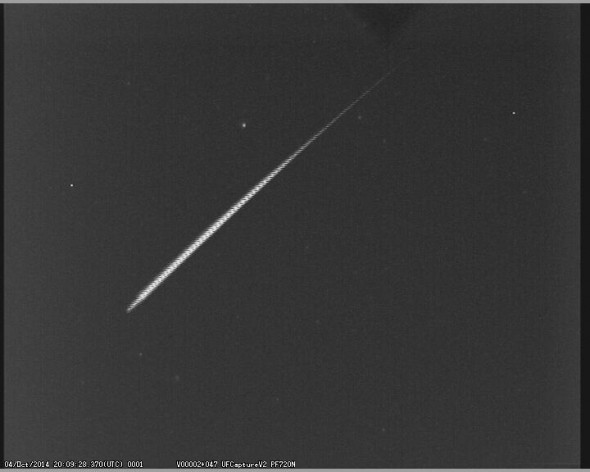
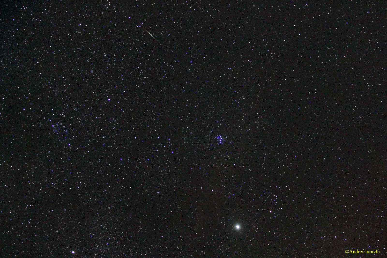
A recent fireball captured over the UK on October 4th, 2014. Credit: the UK Meteor Observation Network.
Mid- to late October is fireball season, a time when several key meteor showers experience a broad peak. We’re already seeing an uptick in fireball activity as monitored by numerous all-sky cameras this month, including NASA’s system positioned across the United States. Three lesser known but fascinating showers are the chief culprits.
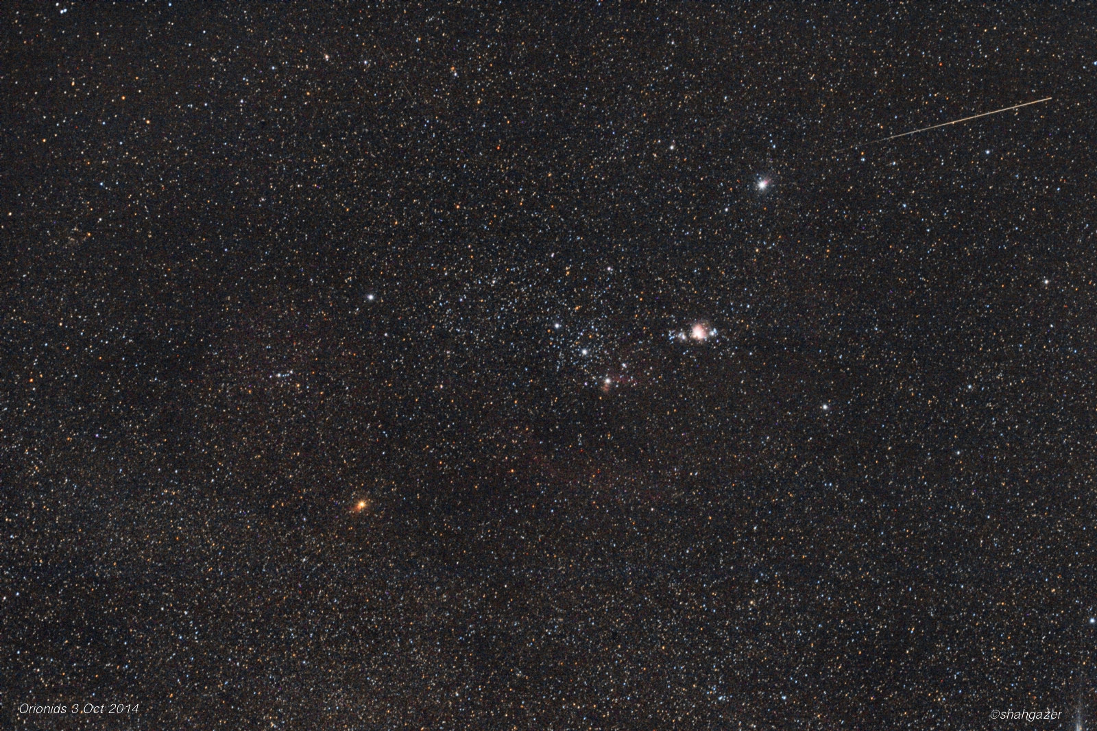
The main meteor shower on tap for the month of October is the Orionids. This shower radiates from the Club of the constellation Orion, and is the product of that most famous comet of them all, 1P Halley. Halley’s Comet is actually the source of two annual meteor showers, the October Orionids and the May Eta Aquarids. We’re seeing the inward stream of Halley debris in October, and Orionid velocities average a swift 66 kilometres a second. The radiant rides highest for northern hemisphere observers at 4 AM local, and 2014 sees an estimated zenithal hourly rate (ZHR) of 20 predicted to arrive on the mornings of October 21st through the 22nd. The Orionids experience a broad peak spanning October 21st through November 7th, and 2014 sees the peak arrive just two days prior to the Moon reaching New phase. The Orionids have exhibited an uptick in activity as high as 50-75 per hour from 2005-2007, and it’s been suggested that a 12 year peak cycle may govern the Orionids, as the path of meteoroid debris stream is modified by the gravitational influence of the giant planet Jupiter.
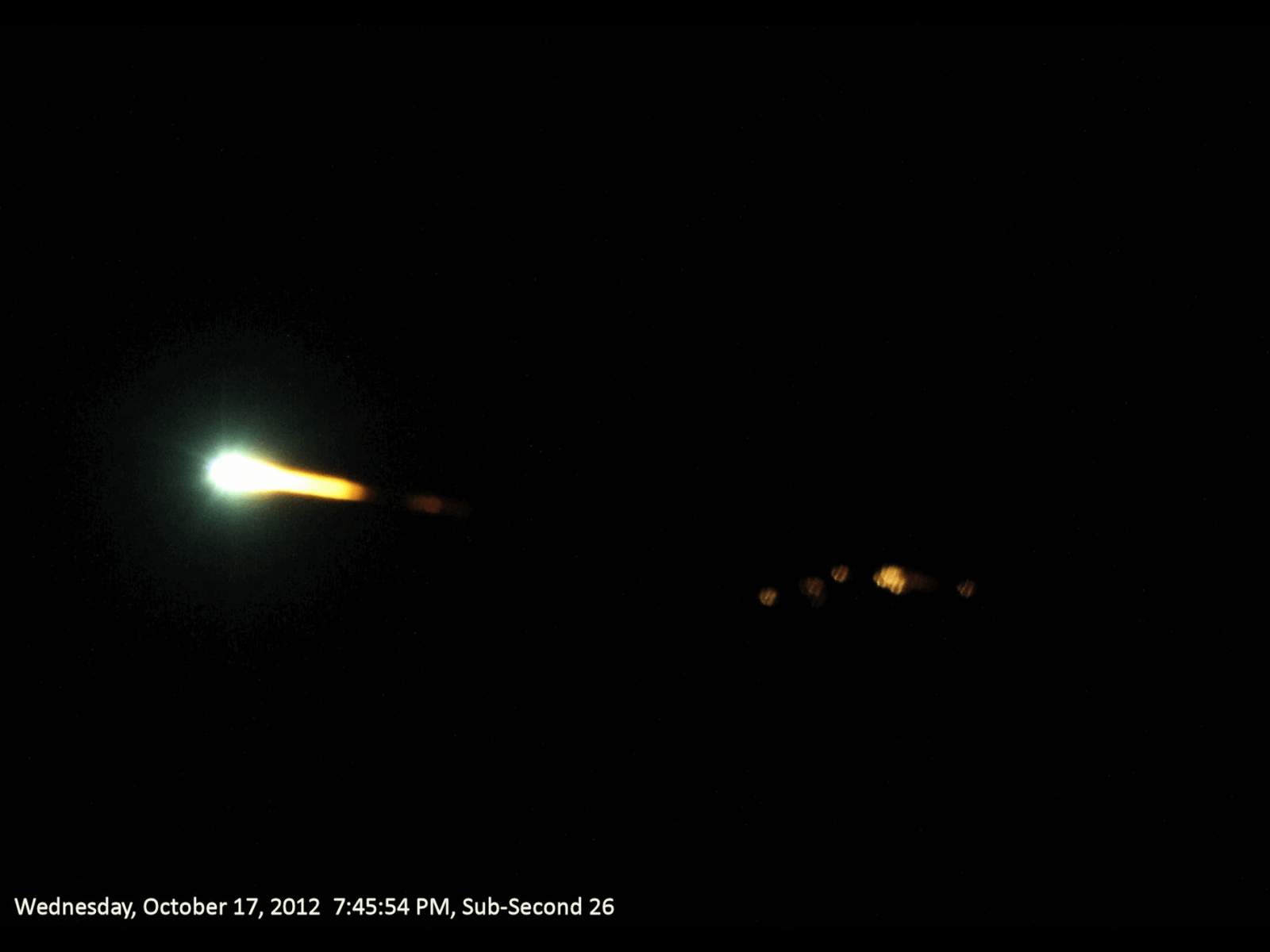
Two other nearby radiants in the sky also produce an exceptionally large number of fireballs in late October: the Southern Taurids and Northern Taurids. These are complex streams laid down by the periodic comet 2P Encke, which possesses the shortest orbital period of any comet known at 3.3 years. Though the ZHR for both is only slightly above the background sporadic rate for northern hemisphere Fall at about five per hour, the Taurids also produce a high ratio of fireballs. The southern Taurids peak in early October and are already active, and the Northern Taurids peak in late October through early November, earning them the nickname the “Fireballs of Halloween”. Unlike many meteor showers, the Northern Taurids are approaching the Earth from behind in our orbit and have a slow relative atmospheric entry velocity of 28 kilometres per second. This makes for long, stately meteor trains often visible in the evening hours before local midnight.
The Taurids also seem to exhibit a seven year periodicity that begs for further study. 2008 was a fine year for Taurid fireballs… could 2015 be next?
Of course, the exact definition of a “fireball” meteor varies by source, though we prefer the definition of a fireball as a meteor brighter than magnitude -3. A fireball reaching -14 (a Full Moon equals magnitude -13, about 2.5 times fainter) is often termed a bolide.
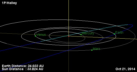
Comet 1P/Halley’s orbital path through the inner solar system. (Credit: NASA/JPL).
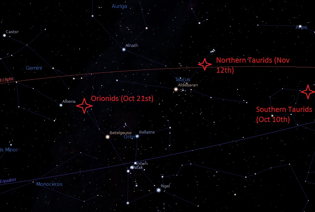
The positions of the radiants of the Orionids and the Taurids, with peak dates. Credit: Stellarium.
Spot a fireball? The American Meteor Society maintains a great online database of recent sightings and reports. Keep in mind, lots of “meteor-wrongs” inevitably crop up on Facebook and Twitter during any event, posted by folks eager for likes and retweets. Faves of such spoofers are: the Peekskill meteor train, the reentry of Hyabusa, Mir, and scenes (!) from the movie Armageddon. We’ve seen ‘em all passed off as legit, though you’re more than welcome to try and be original… a majority of initial meteor images almost always come from dash cams (remember Chelyabinsk?) and security cameras.
Finally, in addition to fireballs, there’s another astronomical tie-in for Halloween, as it’s one of four cross-quarter tie-in days approximately mid-way between a solstice and an equinox. The other three are: Lammas Day (August 1st), Groundhog’s Day (February 2nd) and May Day (May 1st). We just think that it’s great — if a bit paradoxical — to see modern day suburbanites dress up as ghouls and goblins as they reenact archaic rites and holidays…
Don’t forget to keep an eye out for the fireballs of October this Halloween!

About David Dickinson
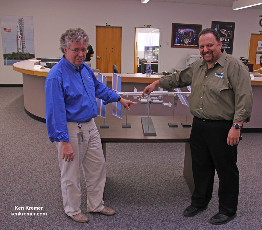
David Dickinson is an Earth science teacher, freelance science writer, retired USAF veteran & backyard astronomer. He currently writes and ponders the universe from Tampa Bay, Florida.- FASHION WEEK - USA Fashion and Music News
- GOOGLE NEWS - Google News Blogger
- PINTEREST ACROSS THE UNIVERSE - Google Images Nasa Images
- LAST FM - Download Music Legally Direct From Artist
- WOMEN COMMUNITY - Women Communty Photography Videos Beauty
- DISNEY CHANNEL - Photos and Music News
- BABY JUSTIN BIEBER - Google Images Google News
- LADY GAGA - Google Images Google News
- ACROSS THE UNIVERSE - Google Images Universe Pictures
- VICTORIA´S SECRET COMMUNITY - Victoria´s Secret Fashion Show Photos


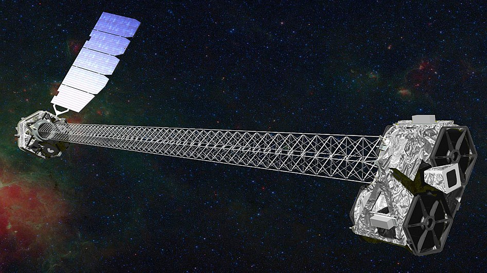
![An illustration [click for video] of a rotation neutron star, the remnants of a super nova explosion has been found to be an ultraluminous X-ray source, the first of its kind. (Credit: NASA, Caltech-JPL)](https://lh3.googleusercontent.com/blogger_img_proxy/AEn0k_tG_pmNpMbkf2N__AXtQnfyxswzqyH_QbXk9cexID4oskHbb7chNw41wfJV17TQKxaohoasVUOuuFUvnXuFGtrqnOxn_g7p-Ki7qRomLlBdnxzpOWCvrqypKPLBL4JvKuTBOyyyDa6_83M_RWzTGDo5IdOlZiPwgd9ew87XVw8BM-dfsd4kQvUPLEpSVWQQXmAwd4zt27J1_YtZeMgWttO0BFOopwI=s0-d)