Defining Life II: Metabolism and Evolution as clues to Extraterrestrial Life

Defining Life II: Metabolism and Evolution as clues to Extraterrestrial Life:

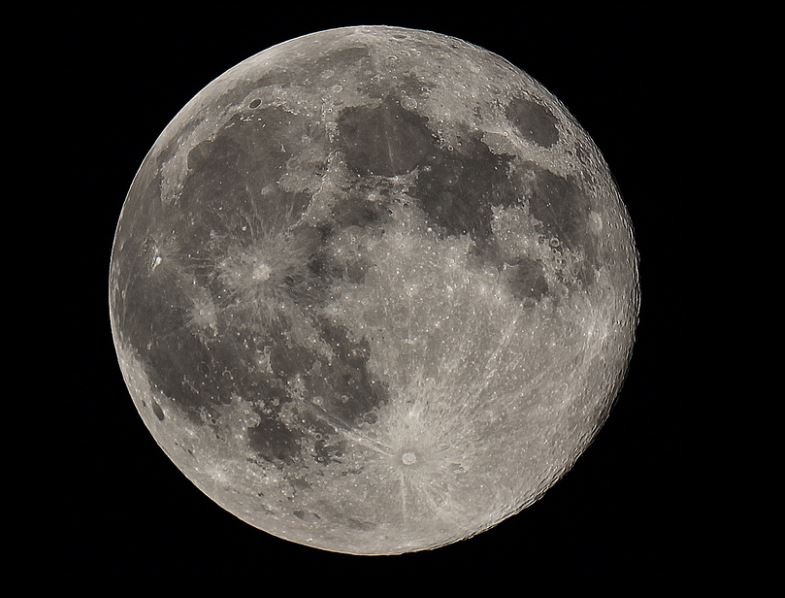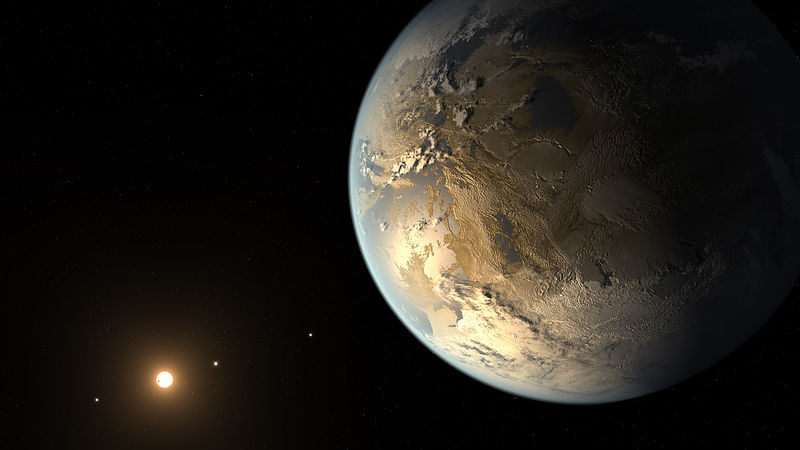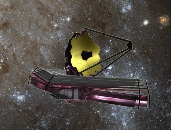
The James Webb Space Telescope, scheduled for launch in 2018, may be the first to be capable of detecting biomarker gases in the atmospheres of extrasolar planets. When an exoplanet passes between its star and Earth, an event called a transit, light that has passed through the planet’s atmosphere can be detected from a vantage point near Earth. When light passes through the exoplanet’s atmosphere, some wavelengths are absorbed and others transmitted. By analyzing the transmitted light spectrum, astronomers can learn the composition of the planet’s atmosphere. Astrobiologists hope to find biomarker gases indicating the metabolic waste products of life. The oxygen in Earth’s atmosphere is a waste product of photosynthesis in plants and bacteria. The Webb telescope may be capable of conducting this test for planets larger than Earth (super-earths) transiting small stars. Space telescopes capable of conducting such research on a larger scale have been delayed by budget cuts.

Credit: NASA

In the movie “Avatar”, we could tell at a glance that the alien moon Pandora was teeming with alien life. Here on Earth though, the most abundant life is not the plants and animals that we are familiar with. The most abundant life is simple and microscopic. There are 50 million bacterial organisms in a single gram of soil, and the world wide bacterial biomass exceeds that of all plants and animals. Microbes can grow in extreme environments of temperature, salinity, acidity, radiation, and pressure. The most likely form in which we will encounter life elsewhere in our solar system is microbial.



Astrobiologists need strategies for inferring the presence of alien microbial life or its fossilized remains. They need strategies for inferring the presence of alien life on the distant planets of other stars, which are too far away to explore with spacecraft in the foreseeable future. To do these things, they long for a definition of life, that would make it possible to reliably distinguish life from non-life.

Unfortunately, as we saw in the first installment of this series, despite enormous growth in our knowledge of living things, philosophers and scientists have been unable to produce such a definition. Astrobiologists get by as best they can with definitions that are partial, and that have exceptions. Their search is geared to the features of life on Earth, the only life we currently know.

In the first installment, we saw how the composition of terrestrial life influences the search for extraterrestrial life. Astrobiologists search for environments that once contained or currently contain liquid water, and that contain complex molecules based on carbon. Many scientists, however, view the essential features of life as having to do with its capacities instead of its composition.

In 1994, a NASA committee adopted a definition of life as a “self-sustaining chemical system capable of Darwinian evolution”, based on a suggestion by Carl Sagan. This definition contains two features, metabolism and evolution, that are typically mentioned in definitions of life.

Metabolism is the set of chemical processes by which living things actively use energy to maintain themselves, grow, and develop. According to the second law of thermodynamics, a system that doesn’t interact with its external environment will become more disorganized and uniform with time. Living things build and maintain their improbable, highly organized state because they harness sources of energy in their external environment to power their metabolism.

Plants and some bacteria use the energy of sunlight to manufacture larger organic molecules out of simpler subunits. These molecules store chemical energy that can later be extracted by other chemical reactions to power their metabolism. Animals and some bacteria consume plants or other animals as food. They break down complex organic molecules in their food into simpler ones, to extract their stored chemical energy. Some bacteria can use the energy contained in chemicals derived from non-living sources in the process of chemosynthesis.

In a 2014 article in Astrobiology, Lucas John Mix, a Harvard evolutionary biologist, referred to the metabolic definition of life as Haldane Life after the pioneering physiologist J. B. S. Haldane. The Haldane life definition has its problems. Tornadoes and vorticies like Jupiter’s Great Red Spot use environmental energy to sustain their orderly structure, but aren’t alive. Fire uses energy from its environment to sustain itself and grow, but isn’t alive either.

Despite its shortcomings, astrobiologists have used Haldane definition to devise experiments. The Viking Mars landers made the only attempt so far to directly test for extraterrestrial life, by detecting the supposed metabolic activities of Martian microbes. They assumed that Martian metabolism is chemically similar to its terrestrial counterpart.

One experiment sought to detect the metabolic breakdown of nutrients into simpler molecules to extract their energy. A second aimed to detect oxygen as a waste product of photosynthesis. A third tried to show the manufacture of complex organic molecules out of simpler subunits, which also occurs during photosynthesis. All three experiments seemed to give positive results, but many researchers believe that the detailed findings can be explained without biology, by chemical oxidizing agents in the soil.

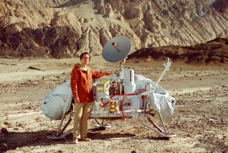
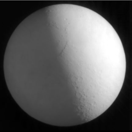
In 1976, two Viking spacecraft landed on Mars. The image is of a model of the Viking lander, along with astronomer and pioneering astrobiologist Carl Sagan. Each lander was equipped with life detection experiments designed to detect life based on its metabolic activities. These activities were assumed to be chemically similar to those of Earthly organisms. The three experiments included: 1) The labeled release experiment, in which radioactively labeled organic nutrients were added to Martian soil. If organisms were present, it was assumed that their metabolism would involve breaking down the nutrients for their energy content and releasing labeled carbon dioxide as a waste product. 2) The gas exchange experiment, in which Martian soil was provided with nutrients and light and monitored for the release of oxygen. On Earth, organisms that capture the energy of sunlight through the process of photosynthesis, like plants and some bacteria, release oxygen as a waste product. 3) The pyrolytic release experiment, in which Martian soil was placed in a chamber with radioactively labeled carbon dioxide. If there were organisms in the soil that photosynthesized like those on Earth, their metabolic processes would take up the gas and use the energy of sunlight to manufacture more complex organic molecules. Radioactive carbon would be given off when those more complex molecules were broken down by heating the sample. All three experiments produced what seemed like positive results. However, most scientists rejected this interpretation because the details of many of the results could be explained by supposing that there were chemical oxidizing agents in the soil instead of life, and because Viking failed to detect organic materials in Martian soil. This interpretation, especially for the labeled release experiment, remains controversial to this day and may need to be revisited based on recent findings.

Credits: NASA/Jet Propulsion Laboratory, Caltech

Some of the Viking results remain controversial to this day. At the time, many researchers felt that the failure to find organic materials in Martian soil ruled out a biological interpretation of the metabolic results. The more recent finding that Martian soil actually does contain organic molecules that might have been destroyed by perchlorates during the Viking analysis, and that liquid water was once abundant on the surface of Mars lend new plausibility to the claim that Viking may have actually succeeded in detecting life. By themselves, though, the Viking results didn’t prove that life exists on Mars nor rule it out.

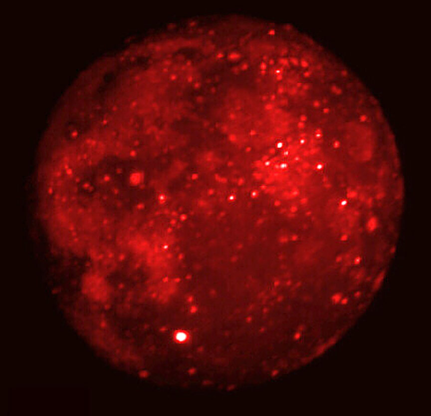
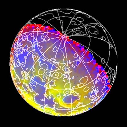
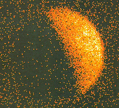
The metabolic activities of life may also leave their mark on the composition of planetary atmospheres. In 2003, the European Mars Express spacecraft detected traces of methane in the Martian atmosphere. In December 2014, a team of NASA scientists reported that the Curiosity Mars rover had confirmed this finding by detected atmospheric methane from the Martian surface.

Most of the methane in Earth’s atmosphere is released by living organisms or their remains. Subterranean bacterial ecosystems that use chemosynthesis as a source of energy are common, and they produce methane as a metabolic waste product. Unfortunately, there are also non-biological geochemical processes that can produce methane. So, once more, Martian methane is frustratingly ambiguous as a sign of life.

Extrasolar planets orbiting other stars are far too distant to visit with spacecraft in the foreseeable future. Astrobiologists still hope to use the Haldane definition to search for life on them. With near future space telescopes, astronomers hope to learn the composition of the atmospheres of these planets by analyzing the spectrum of light wavelengths reflected or transmitted by their atmospheres. The James Webb Space Telescope scheduled for launch in 2018, will be the first to be useful in this project. Astrobiologists want to search for atmospheric biomarkers; gases that are metabolic waste products of living organisms.

Once more, this quest is guided by the only example of a life-bearing planet we currently have; Earth. About 21% of our home planet’s atmosphere is oxygen. This is surprising because oxygen is a highly reactive gas that tends to enter into chemical combinations with other substances. Free oxygen should quickly vanish from our air. It remains present because the loss is constantly being replaced by plants and bacteria that release it as a metabolic waste product of photosynthesis.

Traces of methane are present in Earth’s atmosphere because of chemosynthetic bacteria. Since methane and oxygen react with one another, neither would stay around for long unless living organisms were constantly replenishing the supply. Earth’s atmosphere also contains traces of other gases that are metabolic byproducts.

In general, living things use energy to maintain Earth’s atmosphere in a state far from the thermodynamic equilibrium it would reach without life. Astrobiologists would suspect any planet with an atmosphere in a similar state of harboring life. But, as for the other cases, it would be hard to completely rule out non-biological possibilities.

Besides metabolism, the NASA committee identified evolution as a fundamental ability of living things. For an evolutionary process to occur there must be a group of systems, where each one is capable of reliably reproducing itself. Despite the general reliability of reproduction, there must also be occasional random copying errors in the reproductive process so that the systems come to have differing traits. Finally, the systems must differ in their ability to survive and reproduce based on the benefits or liabilities of their distinctive traits in their environment. When this process is repeated over and over again down the generations, the traits of the systems will become better adapted to their environment. Very complex traits can sometimes evolve in a step-by-step fashion.

Mix named this the Darwin life definition, after the nineteenth century naturalist Charles Darwin, who formulated the theory of evolution. Like the Haldane definition, the Darwin life definition has important shortcomings. It has trouble including everything that we might think of as alive. Mules, for example, can’t reproduce, and so, by this definition, don’t count as being alive.

Despite such shortcomings, the Darwin life definition is critically important, both for scientists studying the origin of life and astrobiologists. The modern version of Darwin’s theory can explain how diverse and complex forms of life can evolve from some initial simple form. A theory of the origin of life is needed to explain how the initial simple form acquired the capacity to evolve in the first place.

The chemical systems or life forms found on other planets or moons in our solar system might be so simple that they are close to the boundary between life and non-life that the Darwin definition establishes. The definition might turn out to be vital to astrobiologists trying to decide whether a chemical system they have found really qualifies as a life form. Biologists still don’t know how life originated. If astrobiologists can find systems near the Darwin boundary, their findings may be pivotally important to understanding the origin of life.

Can astrobiologists use the Darwin definition to find and study extraterrestrial life? It’s unlikely that a visiting spacecraft could detect to process of evolution itself. But, it might be capable of detecting the molecular structures that living organisms need in order to take part in an evolutionary process. Philosopher Mark Bedau has proposed that a minimal system capable of undergoing evolution would need to have three things: 1) a chemical metabolic process, 2) a container, like a cell membrane, to establish the boundaries of the system, and 3) a chemical “program” capable of directing the metabolic activities.

Here on Earth, the chemical program is based on the genetic molecule DNA. Many origin-of-life theorists think that the genetic molecule of the earliest terrestrial life forms may have been the simpler molecule ribonucleic acid (RNA). The genetic program is important to an evolutionary process because it makes the reproductive copying process stable, with only occasional errors.

Both DNA and RNA are biopolymers; long chainlike molecules with many repeating subunits. The specific sequence of nucleotide base subunits in these molecules encodes the genetic information they carry. So that the molecule can encode all possible sequences of genetic information it must be possible for the subunits to occur in any order.

Steven Benner, a computational genomics researcher, believes that we may be able to develop spacecraft experiments to detect alien genetic biopolymers. He notes that DNA and RNA are very unusual biopolymers because changing the sequence in which their subunits occur doesn’t change their chemical properties. It is this unusual property that allows these molecules to be stable carriers of any possible genetic code sequence.

DNA and RNA are both polyelectrolytes; molecules with regularly repeating areas of negative electrical charge. Benner believes that this is what accounts for their remarkable stability. He thinks that any alien genetic biopolymer would also need to be a polyelectrolyte, and that chemical tests could be devised by which a spacecraft might detect such polyelectrolyte molecules. Finding the alien counterpart of DNA is a very exciting prospect, and another piece to the puzzle of identifying alien life.

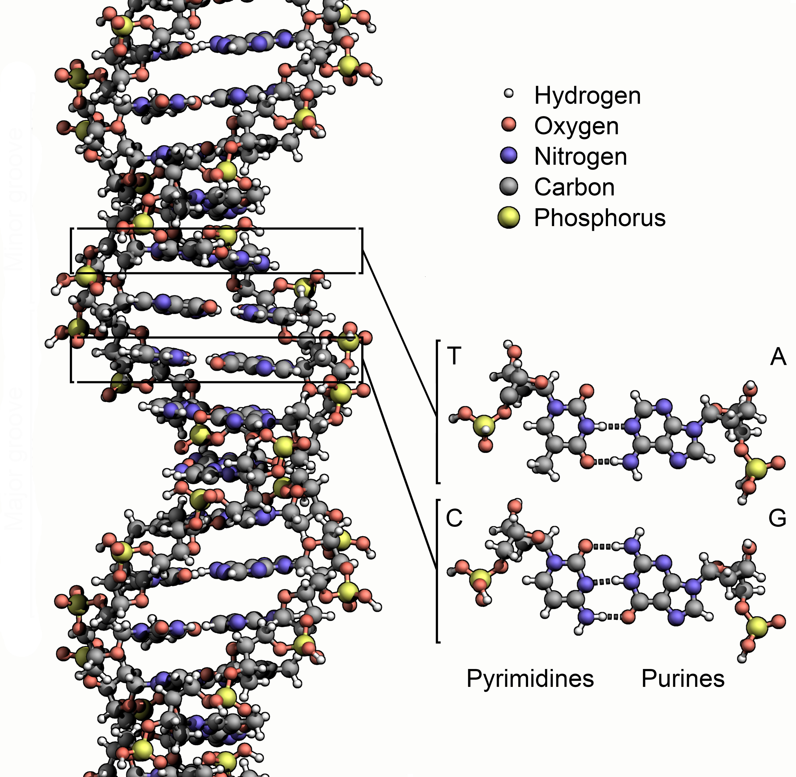
Deoxyribonucleic acid (DNA) is the genetic material for all known life on Earth. DNA is a biopolymer consisting of a string of subunits. The subunits consist of nucleotide base pairs containing a purine (adenine A, or guanine G) and a pyrimidine (thymine T, or cytosine C). DNA can contain nucleotide base pairs in any order without its chemical properties changing. This property is rare in biopolymers, and makes it possible for DNA to encode genetic information in the sequence of its base pairs. This stability is due to the fact that each base pair contains phosphate groups (consisting of phosphorus and oxygen atoms) on the outside with a net negative charge. These repeated negative charges make DNA a polyelectrolyte. Computational genomics researcher Steven Benner has hypothesized that alien genetic material will also be a polyelectrolyte biopolymer, and that chemical tests could therefore be devised to detect alien genetic molecules.

Credit: Zephyris

In 1996 President Clinton, made a dramatic announcement of the possible discovery of life on Mars. Clinton’s speech was motivated by the findings of David McKay’s team with the Alan Hills meteorite. In fact, the McKay findings turned out to be just one piece to the larger puzzle of possible Martian life. Unless an alien someday ambles past our waiting cameras, the question of whether or not extraterrestrial life exists is unlikely to be settled by a single experiment or a sudden dramatic breakthrough. Philosophers and scientists don’t have a single, sure-fire definition of life. Astrobiologists consequently don’t have a single sure-fire test that will settle the issue. If simple forms of life do exist on Mars, or elsewhere in the solar system, it now seems likely that that fact will emerge gradually, based on many converging lines of evidence. We won’t really know what we’re looking for until we find it.

References and further reading:

P. S. Anderson (2011) Could Curiosity Determine if Viking Found Life on Mars?, Universe Today.

S. K. Atreya, P. R. Mahaffy, A-S. Wong, (2007), Methane and related trace species on Mars: Origin, loss, implications for life, and habitability, Planetary and Space Science, 55:358-369.

M. A. Bedau (2010), An Aristotelian account of minimal chemical life, Astrobiology, 10(10): 1011-1020.

S. A. Benner (2010), Defining life, Astrobiology, 10(10):1021-1030.

E. Machery (2012), Why I stopped worrying about the definition of life…and why you should as well, Synthese, 185:145-164.

G. M. Marion, C. H. Fritsen, H. Eicken, M. C. Payne, (2003) The search for life on Europa: Limiting environmental factors, potential habitats, and Earth analogs. Astrobiology 3(4):785-811.

L. J. Mix (2015), Defending definitions of life, Astrobiology, 15(1) posted on-line in advance of publication.

P. E. Patton (2014) Moons of Confusion: Why Finding Extraterrestrial Life may be Harder than we Thought, Universe Today.

T. Reyes (2014) NASA’s Curiosity Rover detects Methane, Organics on Mars, Universe Today.

S. Seeger, M. Schrenk, and W. Bains (2012), An astrophysical view of Earth-based biosignature gases. Astrobiology, 12(1): 61-82.

S. Tirard, M. Morange, and A. Lazcano, (2010), The definition of life: A brief history of an elusive scientific endeavor, Astrobiology, 10(10):1003-1009.

C. R. Webster, and numerous other members of the MSL Science team, (2014) Mars methane detection and variability at Gale crater, Science, Science express early content.

Did Viking Mars landers find life’s building blocks? Missing piece inspires new look at puzzle. Science Daily Featured Research Sept. 5, 2010

NASA rover finds active and ancient organic chemistry on Mars, Jet Propulsion laboratory, California Institute of Technology, News, Dec. 16, 2014.

About Paul Patton

Paul Patton is a freelance science writer. He holds a Bachelor's degree in physics from the University of Wisconsin Green Bay, a Master's degree in the history and philosophy of science from Indiana University, and a Doctorate in neuroscience from the University of Chicago. He has been interested in space, astronomy, and extraterrestrial life since early childhood.

• FASHION WEEK - USA Fashion and Music News
• GOOGLE NEWS - Google News Blogger
• PALCO MP3 - Download Music Legally Direct From Artist
• LAST FM - Download Music Legally Direct From Artist
• USA FASHION - Fashion In USA Photography Videos Beauty
• DISNEY CHANNEL - Photos and Music News
• BABY JUSTIN BIEBER - Google Images Google News
• LADY GAGA  - Google Images Google News
• UNIVERSE PICTURES - Google Images Nature Pictures
• VICTORIA´S SECRET Google + - Victoria´s Secret Fashion Show Photos

How Did We Find the Distance to the Sun?

How Did We Find the Distance to the Sun?:

Credit: NASA Goddard Space Flight Center

How far is the Sun? It seems as if one could hardly ask a more straightforward question. Yet this very inquiry bedeviled astronomers for more than two thousand years.

Certainly it’s a question of nearly unrivaled importance, overshadowed in history perhaps only by the search for the size and mass of the Earth. Known today as the astronomical unit, the distance serves as our reference within the solar system and the baseline for measuring all distances in the Universe.

Thinkers in Ancient Greece were among the first to try and construct a comprehensive model of the cosmos. With nothing but naked-eye observations, a few things could be worked out. The Moon loomed large in the sky so it was probably pretty close. Solar eclipses revealed that the Moon and Sun were almost exactly the same angular size, but the Sun was so much brighter that perhaps it was larger but farther away (this coincidence regarding the apparent size of the Sun and Moon has been of almost indescribable importance in advancing astronomy). The rest of the planets appeared no larger than the stars, yet seemed to move more rapidly; they were likely at some intermediate distance. But, could we do any better than these vague descriptions? With the invention of geometry, the answer became a resounding yes.

The first distance to be measured with any accuracy was that of the Moon. In the middle of the 2nd century BCE, Greek astronomer Hipparchus pioneered the use of a method known as parallax. The idea of parallax is simple: when objects are observed from two different angles, closer objects appear to shift more than do farther ones. You can demonstrate this easily for yourself by holding a finger at arm’s length and closing one eye and then the other. Notice how your finger moves more than things in the background? That’s parallax! By observing the Moon from two cities a known distance apart, Hipparchus used a little geometry to compute its distance to within 7% of today’s modern value – not bad!

The Moon was the first object whose distance was accurately measured. Credit and copyright: James Lennie.

With the distance to the Moon known, the stage was set for another Greek astronomer, Aristarchus, to take the first stab at determining the Earth’s distance from the Sun. Aristarchus realized that when the Moon was exactly half illuminated, it formed a right triangle with the Earth and the Sun. Now knowing the distance between the Earth and the Moon, all he needed was the angle between the Moon and Sun at this moment to compute the distance of the Sun itself. It was brilliant reasoning undermined by insufficient observations. With nothing but his eyes to go on, Aristarchus estimated this angle to be 87 degrees, not terribly far from the true value of 89.83 degrees. But when the distances involved are enormous, small errors can be quickly magnified. His result was off by a factor of more than a thousand.

Over the next two thousand years, better observations applied to Aristarchus’ method would bring us within 3 or 4 times the true value. So how could we improve this further? There was still only one method of directly measuring distance and that was parallax. But, finding the parallax of the Sun was far more challenging than that of the Moon. After all, the Sun is essentially featureless and its incredible brightness obliterates any view we might have of the stars that lurk behind. What could we do?

By the eighteenth century, however, our understanding of the world had progressed substantially. The field of physics was now in its infancy and it provided a critical clue. Johannes Kepler and Isaac Newton had shown that the distances between the planets were all related; find one and you would know them all. But would any be easier to find than the Earth’s? It turns out that the answer is yes. Sometimes. If you’re lucky.

The key is the transit of Venus. During a transit, the planet crosses in front of the Sun as seen from Earth. From different locations, Venus will appear to cross larger or smaller parts of the Sun. By timing how long these crossings take, James Gregory and Edmond Halley realized that the distance to Venus (and hence the Sun) could be determined (Interested in the nitty gritty of how this is done? NASA has a pretty nice explanation available here.). Now’s the time when I’d usually say something like: Seems pretty straightforward, right? There’s only one catch… But perhaps that’s never been more untrue. The odds were so stacked against success that it’s truly a testament to the importance of this measurement that anyone even attempted it.

An astronomer traveling with Capt. James Cook observed the 1769 transit of Venus from Tahiti.

First off, transits of Venus are extremely rare. Like once-in-a-lifetime rare (although they do come in pairs). By the time Halley realized that this method would work, he knew that he was too old to have a chance to complete it himself. So, in hope that a future generation would undertake the task, he wrote out specific instructions on how the observations must be carried out. In order for the end result to have the desired accuracy, the timing of the transit needed to be measured down to the second. In order to have a large separation in distance, the observing sites would need to be located at the far reaches of the Earth. And, in order to ensure that cloudy weather didn’t ruin the chance of success, observers would be needed at locations all over the globe. Talk about a big undertaking in an era when transcontinental travel could take years.

Despite these challenges, astronomers in France and England resolved that they would collect the necessary data during the 1761 transit. By that time, however, the situation was even worse: England and France were embroiled in the Seven Years’ War. Travel by sea was nearly impossible. Nevertheless, the effort persisted. Although not all observers were successful (clouds blocked some, warships others), when combined with data collected during another transit eight years later, the undertaking had been a success. French astronomer Jerome Lalande collected all the data and computed the first accurate distance to the Sun: 153 million kilometers, good to within three percent of the true value!

A brief aside: the number we’re talking about here is called the Earth’s semi-major axis, meaning that it’s the average distance between the Earth and the Sun. Because the Earth’s orbit isn’t perfectly round, we actually get about 3% closer and farther throughout the course of a year. Also, like many numbers in modern science, the formal definition of the astronomical unit has been altered a bit. As of 2012, 1 AU = 149,597,870,700 meters exactly, regardless of whether we find the Earth’s semi-major axis is slightly different in the future.

Since the groundbreaking observations made during the transit of Venus, we’ve refined our knowledge of the Earth-Sun distance tremendously. We’ve also used it to unlock an understanding of the vastness of the Universe. Once we knew how large the Earth’s orbit was, we could use parallax to measure the distance to other stars by making observations spaced out by six months (when the Earth has travelled to the other side of the Sun, a distance of 2 AU!). This revealed a cosmos that stretched on unendingly and would eventually lead to the discovery that our universe is billions of years old. Not bad for asking a straightforward question!

About Morgan Rehnberg

Morgan Rehnberg studies astrophysics and planetary science as a graduate student at the University of Colorado - Boulder. When he's not plumbing the depths of Saturn's rings, he advocates for greater public engagement with science.

• FASHION WEEK - USA Fashion and Music News
• GOOGLE NEWS - Google News Blogger
• PINTEREST USA FASHION - Models Top Models Supermodels Fashion
• LAST FM - Download Music Legally Direct From Artist
• USA FASHION - USA Fashion Google + Photography Videos Beauty
• DISNEY CHANNEL - Photos Music News
• BABY JUSTIN BIEBER - Google Images Google News
• LADY GAGA  - Google Images Google News
• UNIVERSE PICTURES - Google Images Nature Pictures
• VICTORIA´S SECRET - Google + Victoria´s Secret Fashion Show Photos

Good Morning, Space Station … A Dragon Soars Soon!

Good Morning, Space Station … A Dragon Soars Soon!:

Commander Barry “Butch” Wilmore on the International Space Station shared this beautiful image of #sunrise earlier today, 1/3/15. Credit: NASA/Barry ‘Butch’ Wilmore

Good Morning, Space Station!

It’s sunrise from space – one of 16 that occur daily as the massive lab complex orbits the Earth about every 90 minutes while traveling swiftly at about 17,500 mph from an altitude of about 250 miles (400 kilometers).



Just stare in amazement at this gorgeous sunrise view of ‘Our Beautiful Earth’ taken earlier today, Jan. 3, 2015, aboard the International Space Station (ISS) by crewmate and NASA astronaut Barry “Butch” Wilmore.

And smack dab in the middle is the Canadian-built robotic arm that will soon snatch a soaring Dragon!

Wilmore is the commander of the ISS Expedition 42 crew of six astronauts and cosmonauts hailing from three nations; America, Russia and Italy.

He is accompanied by astronauts Terry Virts from NASA and Samantha Cristoforetti from the European Space Agency (ESA) as well as by cosmonauts Aleksandr Samokutyayev, Yelena Serova, and Anton Shkaplerov from Russia.

All told the crew of four men and two women see 16 sunrises and 16 sunsets each day. During the daylight periods, temperatures reach 200 ºC, while temperatures plunge drastically during the night periods to -200 ºC.

Here’s another beautiful ISS sunset view captured on Christmas by Terry Virts:

Astronaut Terry Virts on the International Space Station shared this beautiful sunrise image on Twitter saying “Sunrise on Christmas morning – better than any present I could ask for!!!!” Credit: NASA/Terry Virts

Virts tweeted the picture and wrote: “Sunrise on Christmas morning – better than any present I could ask for!!!!”

Another treasure from Virts shows the many splendid glorious colors of Earth seen from space but not from the ground:

Sunset Over the Gulf of Mexico

“In space you see intense colors, shades of blue that I’d never seen before,” says NASA astronaut Terry Virts. Credit: NASA/@astro_terry

“In space you see intense colors, shades of blue that I’d never seen before,” says Virts from his social media accounts (http://instagram.com/astro_terry/) (http://instagram.com/iss).

“It’s been said a thousand times but it’s true: There are no borders that you can see from space, just one beautiful planet,” he says. “If everyone saw the Earth through that lens I think it would be a much better place.”

And many of the crews best images are taken from or of the 7 windowed Cupola.

Here’s an ultra cool shot of Butch waving Hi!

“Hi from the cupola!” #AstroButch. Credit: NASA/ISS

And they all eagerly await the launch and arrival of a Dragon! Indeed it’s the SpaceX cargo Dragon currently slated for liftoff in three days on Tuesday, Jan. 6.

Weather odds are currently 60% favorable for launch of the unmanned space station resupply ship on the SpaceX CRS-5 mission.

The launch was postponed from Dec. 19 when a static fire test of the first stage engines on Dec. 17 shut down prematurely.

A second static fire test of the SpaceX Falcon 9 went the full duration of approximately 3 seconds and cleared the path for a liftoff attempt after the Christmas holidays.

New countdown clock at NASA’s Kennedy Space Center displays SpaceX Falcon 9 CRS-5 mission and recent Orion ocean recovery at the Press Site viewing area on Dec. 18, 2014. Credit: Ken Kremer – kenkremer.com

CRS-5 is slated to blast off at 6:20 a.m. EST Tuesday, Jan. 6, 2015, atop a SpaceX Falcon 9 rocket from Cape Canaveral Air Force Station in Florida.

NASA Television live launch coverage begins at 5 a.m. EST.

Assuming all goes well, Dragon will rendezvous at the ISS on Thursday, Jan. 8, for grappling and berthing by the astronauts maneuvering the 57 foot-long (22 m) Canadian built robotic arm.

Remember that you can always try and catch of glimpse of the ISS flying overhead by checking NASA’s Spot the Station website with a complete list of locations.

It’s easy to plug in and determine visibilities in your area worldwide.

And don’t forget to catch up on the Christmas holiday and New Year’s 2015 imagery and festivities from the station crews in my recent stories - here, here and here.

Stay tuned here for Ken’s continuing Earth and planetary science and human spaceflight news.

Ken Kremer

Happy New Year! Celebrating from space with @AstroTerry. Credit: NASA/Terry Virts

ISS Expedition 42. Credit: NASA/ESA/Roscosmos

About Ken Kremer

Dr. Ken Kremer is a speaker, scientist, freelance science journalist (Princeton, NJ) and photographer whose articles, space exploration images and Mars mosaics have appeared in magazines, books, websites and calendars including Astronomy Picture of the Day, NBC, BBC, SPACE.com, Spaceflight Now and the covers of Aviation Week & Space Technology, Spaceflight and the Explorers Club magazines. Ken has presented at numerous educational institutions, civic & religious organizations, museums and astronomy clubs. Ken has reported first hand from the Kennedy Space Center, Cape Canaveral, NASA Wallops, NASA Michoud/Stennis/Langley and on over 40 launches including 8 shuttle launches. He lectures on both Human and Robotic spaceflight - www.kenkremer.com. Follow Ken on Facebook and Twitter

• FASHION WEEK - USA Fashion and Music News
• GOOGLE NEWS - Google News Blogger
• PALCO MP3 - Download Music Legally Direct From Artist
• LAST FM - Download Music Legally Direct From Artist
• USA FASHION - Fashion In USA Photography Videos Beauty
• DISNEY CHANNEL - Photos and Music News
• BABY JUSTIN BIEBER - Google Images Google News
• LADY GAGA  - Google Images Google News
• UNIVERSE PICTURES - Google Images Nature Pictures
• VICTORIA´S SECRET Google + - Victoria´s Secret Fashion Show Photos

Rogue Star HIP 85605 on Collision Course with our Solar System, but Earthlings Need Not Worry

Rogue Star HIP 85605 on Collision Course with our Solar System, but Earthlings Need Not Worry:

Our Solar System is due for a near-collision with HIP 85605, a star 16 light-years away, in roughly 40,000 years. Credit: Dana Berry, SkyWorks Digital, Inc.

It’s known as HIP 85605, one of two stars that make up a binary in the Hercules constellation roughly 16 light years away. And if a recent research paper produced by Dr. Coryn Bailer-Jones of the Max Planck Institute for Astronomy in Heidelberg, Germany is correct, it is on a collision course with our Solar System.

Now for the good news: according to Bailer-Jones’ calculations, the star will pass by our Solar System at a distance of 0.04 parsecs, which is equivalent to 8,000 times the distance between the Earth and the Sun (8,000 AUs). In addition, this passage will not affect Earth or any other planet’s orbit around the Sun. And perhaps most importantly of all, none of it will be happening for another 240,000 to 470,000 years from now.

“Even though the galaxy contains very many stars,” Bailor-Jones told Universe Today via email, “the spaces between them are huge. So even over the (long) life of our galaxy so far, the probability of any two stars have actually collided — as opposed to just coming close — is extremely small.”

However, in astronomical terms, that still counts as a near-miss. In a universe that is 46 billion light years in any direction – and that’s just the observable part of it – an event that is expected to take place just 50 light days away is considered to be pretty close. And in the context of space and time, a quarter of a million to half a million years is the very near future.

The real concern is the effect that the passage of HIP 85605 could have on the Oort Cloud – the massive cloud of icy planetesimals that surrounds the Solar System. Given that it’s distance is between 20,000 and 50,000 AU from our Sun, HIP 85605 would actually move through the Oort cloud and cause serious disruption.

The layout of the Solar System, including the Oort Cloud, which lies 50,000 AU from our Sun. Credit: NASA

Many of these planetesimals could be blown off into space, but others could be sent hurtling towards Earth. Assuming humanity is still around at this point in time, this could present a bit of an inconvenience, even if it is spread over the course of a million years.

As it stands, such “close encounters” between stars are quite rare. Stellar collisions usually only occur within binaries, where white dwarfs or neutron stars are concerned. “The exception to this is physically bound binary stars in a tight orbit,” said Bailor-Jones. “It can and does happen that one star expands during its evolution and will then interfere with the evolution of the other star. Neutron-neutron star pairs can even merge.”

But of course, on an astronomical timescale, stars passing each other by as they perform their cosmic dance is actually a pretty common occurrence. As part of Bailer-Jones larger study of over 50,000 stars within our galaxy, this “close encounter”  is one of several predicted to take place in the coming years.

Of all of them, only HIP 85605 is expected to come within a single parsec between 240 and 470 thousand years from now. He also indicates with (90% confidence) that the last time such an encounter took place was 3.8 million years ago when gamma Microscopii – a G7 giant which has two and a half times the mass of our Sun – came within 0.35-1.34 pc of our system, which may have caused a large perturbation in the Oort cloud.

Tightly bound binary stars, like the ones illustrated here, sometimes result in stellar collisions. Credit: Chandra

On his MPIA webpage, in the study’s FAQ section, Bailor-Jones claims that his research into stellar close encounters was motivated by a desire to study the potential impacts of astronomical phenomena on Earth, and is part of a larger program named “astroimpacts”.

“I am interested in the history of the Earth,” he says, “and astronomical phenomena have clearly played a role in this. But what role precisely, how significant, and what can we expect to happen in the future?” Whereas several studies have been conducted in the past, he feels that the methods – which include assuming a linear relative motion of stars – produces inaccurate results.”

In contrast, Bailor-Jones study relies on “more recent data or re-analyses of data to produce hopefully more accurate results, and then compensate more rigorously for the uncertainties in the data, so that I can attach probabilities to my statements.”

As a result of this, he predicts that HIP 85605 has a 90% chance of passing within a single parsec of our Sun in the next 240 to 470 thousands years. However, he also admits that if the astronomy is incorrect, the next closest encounter won’t be happening for another 1.3 million years, when a K7 dwarf known as GL 710 is predicted to pass within 0.10 – 0.44 parsecs.

Bailor-Jones also believes that the European Space Agency’s Gaia spacecraft will help make more accurate predictions in the future. By understanding and mapping the environment of the Milky Way Galaxy, measuring the gravitational potential and determining the velocity of stars, scientists will be able to see how their various orbits around the galaxy’s center could cause them to intersect.

It is likely that passing stars have a system of exoplanets (like Kepler-186f pictured here), which would place them within a few parsecs of Earth. Image Credit: NASA Ames/SETI Institute/JPL-CalTech

But perhaps the most interesting question explored on his webpage is the possibility of using stellar close encounters as a shortcut for exploring exoplanets. According to current cosmological models, the majority of stars within our galaxy are believed to host exoplanets.

So if a star is passing us at just a few parsecs (or even with a single parsec) why not hop on over and investigate its planets? Well, as Bailor-Jones indicates, that’s not really a practical idea: “Traveling to a star passing our solar system at a distance of around 1 pc with a relative speed of 30 km/s is no easier than traveling the the nearby stars (the nearest of which is just over 1 pc away). And we would have to wait 10s of thousands of years for the next encounter. If we can ever achieve interstellar travel, I don’t suppose it would take that long to achieve, so why wait?”

Darn. Still, if there’s one thing this phenomena and Bailor-Jones study reminds us, it is that in the course of dancing around the center of the Milky Way, stars are not fixed in a single point in space. Not only do they periodically move within reach of each other, they can also have an affect on life within them.

Alas, the timescale on which such things happen, not to mention the consequences they entail, are so large that people here on Earth need not worry. By the time HIP 85605 or GL 710 come within a parsec or two of us, we’ll either be long-since dead or too highly evolved to care!

Further Reading: arXiv Astrophysics, Max Planck Institute of Astronomy

About Matt Williams

Author, freelance writer, educator, Taekwon-Do instructor, and loving hubby, son and Island boy!

• FASHION WEEK - USA Fashion and Music News
• GOOGLE NEWS - Google News Blogger
• PINTEREST ACROSS THE UNIVERSE - Google Images Nasa Images
• LAST FM - Download Music Legally Direct From Artist
• WOMEN COMMUNITY - Women Communty Photography Videos Beauty
• DISNEY CHANNEL - Photos and Music News
• BABY JUSTIN BIEBER - Google Images Google News
• LADY GAGA  - Google Images Google News
• ACROSS THE UNIVERSE - Google Images Universe Pictures
• VICTORIA´S SECRET COMMUNITY - Victoria´s Secret Fashion Show Photos

Finding Lovejoy: How to Follow the Path of Comet 2014 Q2 Through January

Finding Lovejoy: How to Follow the Path of Comet 2014 Q2 Through January:

A splendid capture of comet Q2 Lovejoy as it passes near M79 at the end of 2014. Credit and copyright: Andre van der Hoeven.

Have you seen the amazing pics? A bright comet graces evening skies this month, assuring that 2015 is already on track to be a great year for astronomy.

We’re talking about Comet C/2014 Q2 Lovejoy. Discovered by comet hunter extraordinaire Terry Lovejoy on August 17^th, 2014, this denizen of the Oort Cloud has already wowed observers as it approaches its passage perihelion through the inner solar system in the coming week.

First, our story thus far. We’ve been following all Comet Q2 Lovejoy action pretty closely here at Universe Today, from its surreptitious brightening ahead of schedule, to its recent tail disconnection event, to its photogenic passage past the +8.6 magnitude globular cluster Messier 79 (M79) in the constellation Lepus. We also continue to be routinely blown away by reader photos of the comet. And, like the Hare for which Lepus is named, Q2 Lovejoy is now racing rapidly northward, passing into the rambling constellation of Eridanus the River before entering the realm of Taurus the Bull on January 9^th and later crossing the ecliptic plane in Aries.

The path of Comet Q2 Lovejoy from January 2nd to the 31st. Ticks mark the position of the comet at 7PM EST/midnight Universal Time. Credit: Created using Starry Night Education software.

And the best window of opportunity for spying the comet is coming right up. We recently caught our first sight of Q2 Lovejoy a few evenings ago with our trusty Canon 15x 45 image-stabilized binocs from Mapleton, Maine.  Even as seen from latitude 47 degrees north and a frosty -23 Celsius (-10 Fahrenheit) — a far cry from our usual Florida based perspective — the comet was an easy catch as a bright fuzz ball. Q2 Lovejoy was just outside of naked eye visibility for us this week, though I suspect that this will change as the Moon moves out of the evening picture this weekend.

Currently shining at magnitude +5.5, Comet Q2 Lovejoy has already been spied by eagle-eyed observers unaided from dark sky sites to the south. Astrophotographers have revealed its long majestic dust and ion tails, as well as the greenish hue characteristic of bright comets. That green color isn’t kryptonite, but the fluorescing of diatomic carbon and cyanogen gas shed by the comet as it’s struck by ultraviolet sunlight. This greenish color is far more apparent in photographs, though it might just be glimpsed visually if the intrinsic brightness of the coma exceeds expectations. Q2 Lovejoy just passed opposition at 0.48 AU from the Earth today on January 2^nd, and will make its closest passage from our fair world on January 7th at 0.47 AU (43.6 million kilometres) distant.

Comet Q2 Lovejoy via Iphone (!) and a NexStra 8SE telescope. Credit and copyright: Andrew Symes.

What’s so special about the coming week? Well, we also cross a key milestone for evening observing, as the light-polluting Moon reaches Full phase on Sunday January 5^th at 4:54 UT (11:54 PM EDT on the 4^th) and begins sliding out of the evening sky on successive evenings. That’s good news, as Comet Q2 Lovejoy enters the “prime time” evening sky and culminates over the southern horizon at around 10:30 PM local this weekend, then 8:00 PM on January the 15^th, and just before 6:00 PM by January 31^st.

While many comets put on difficult to observe dusk or dawn appearances — the 2013 apparition of another comet, C/2011 L4 PanSTARRS comes to mind — Q2 Lovejoy is well placed this month in the early evening hours.

The current projected peak brightness for Comet Q2 Lovejoy is +4th magnitude right around mid-January. Already, the comet is bright enough and well-placed to the south for northern hemisphere observers that it’s possible to catch astrophotos of the comet along with foreground objects. If you’ve got a tripod mounted DSLR give it a try… it’s as simple as aiming, focusing manually with a wide field of view, and taking 10 to 30 second exposures to see what turns up. Longer shots will call for sky tracking via a barn-door or motorized mount. Binoculars are you friend in your comet-hunting quest, as they can be readily deployed in sub-zero January temps and provide a generous field of view.

Q2 Lovejoy will also pass near the open clusters of the Hyades and the Pleiades through mid-January, and cross into the constellations of Aries and Triangulum by late January before heading northward to pass between the famous Double Cluster in Perseus and the Andromeda Galaxy M31 in February, proving further photo ops.

A comet hung up among the winter trees… Credit and Copyright: Per/Kam75

From there, Q2 Lovejoy is expected to drop below naked eye visibility in late February before passing very near the North Star Polaris and the northern celestial pole at the end of May on its way out of the inner solar system on its 8,000 year journey.

So, although 2014 didn’t produce the touted “comet of the century,” 2015 is already getting off to a pretty good start in terms of comets. We’re out looking nearly every clear night, and the next “big one” could always drop by at anytime… but hopefully, the first discovery baring the name “Comet Dickinson” will merely put on a spectacular show, and not prove to be an extinction level event…

A green New Year’s Eve comet. Credit and Copyright: Roger Hutchinson.

– Got images of Comet Q2 Lovejoy? Send ‘em in to Universe Today.

– Up late looking for comets? Be sure to also check out the Quadrantid meteors this weekend.

-What other comets offer good prospects in 2015? Check out our Top 101 Events for the Year.

About David Dickinson

David Dickinson is an Earth science teacher, freelance science writer, retired USAF veteran & backyard astronomer. He currently writes and ponders the universe from Tampa Bay, Florida.

• FASHION WEEK - USA Fashion and Music News
• GOOGLE NEWS - Google News Blogger
• PALCO MP3 - Download Music Legally Direct From Artist
• LAST FM - Download Music Legally Direct From Artist
• USA FASHION - Fashion In USA Photography Videos Beauty
• DISNEY CHANNEL - Photos and Music News
• BABY JUSTIN BIEBER - Google Images Google News
• LADY GAGA  - Google Images Google News
• UNIVERSE PICTURES - Google Images Nature Pictures
• VICTORIA´S SECRET Google + - Victoria´s Secret Fashion Show Photos

Moonlight Is a Many-Splendored Thing

Moonlight Is a Many-Splendored Thing:

These are all photos of the Moon but photographed in a variety of different wavelengths of light. The images are arranged from longest to shortest wavelength. Top row from left: Moon in radio waves, submillimeter light, mid-infrared, near-infrared. Bottom row: Visual, ultraviolet, X-rays and gamma rays. Credits (top): NRAO-VLA/U. of British Columbia, Mike Kozubel/MSX Project/NASA-Galileo. Bottom: Bob King/Southwest Research Institute/NASA-ROSAT/Dave Thompson-NASA-GFSC

“By the Light of the Silvery Moon” goes the song. But the color and appearance of the Moon depends upon the particular set of eyes we use to see it. Human vision is restricted to a narrow slice of the electromagnetic spectrum called visible light.

With colors ranging from sumptuous violet to blazing red and everything in between, the diversity of the visible spectrum provides enough hues for any crayon color a child might imagine. But as expansive as the visual world’s palette is, it’s not nearly enough to please astronomers’ retinal appetites.

Visible light is a sliver of light’s full range of “colors” which span from kilometers-long, low-energy radio waves (left) to short wavelength, energetic gamma rays. It’s all light, with each color determined by wavelength. Familiar objects along the bottom reference light wave sizes. Visible light waves are about one-millionth of a meter wide. Credit: NASA

Since the discovery of infrared light by William Herschel in 1800 we’ve been unshuttering one electromagnetic window after another. We build telescopes, great parabolic dishes and other specialized instruments to extend the range of human sight.  Not even the atmosphere gets in our way. It allows only visible light, a small amount of infrared and ultraviolet and selective slices of the radio spectrum to pass through to the ground. X-rays, gamma rays and much else is absorbed and completely invisible.

Earth’s atmosphere blocks a good portion of light’s diversity from reaching the ground, the reason we launch rockets and orbiting telescopes into space. Large professional telescopes are often built on mountain tops above much of the denser, lower atmosphere. This expands the viewing “window” into the infrared. Credit: NASA

To peer into these rarified realms, we’ve lofting air balloons and then rockets and telescopes into orbit or simply dreamed up the appropriate instrument to detect them. Karl Jansky’s homebuilt radio telescope cupped the first radio waves from the Milky Way in the early 1930s; by the 1940s  sounding rockets shot to the edge of space detected the high-frequency sizzle of X-rays.  Each color of light, even the invisible “colors”, show us a new face on a familiar astronomical object or reveal things otherwise invisible to our eyes.

So what new things can we learn about the Moon with our contemporary color vision?

Radio Moon

Radio: Made using NRAO’s 140-ft telescope in Green Bank, West Virginia. Blues and greens represent colder areas of the moon and reds are warmer regions. The left half  of Moon was facing the Sun at the time of the observation. The sunlit Moon appear brighter than the shadowed portion because it radiates more heat (infrared light) and radio waves.

Submillimeter Moon

Submillimeter: Taken using the SCUBA camera on the James Clerk Maxwell Telescope in Hawaii. Submillimeter radiation lies between far infrared and microwaves. The Moon appears brighter on one side because it’s being heated by Sun in that direction. The glow comes from submillimeter light radiated by the Moon itself. No matter the phase in visual light, both the submillimeter and radio images always appear full because the Moon radiates at least some light at these wavelengths whether the Sun strikes it or not.

Mid-infrared Moon

Mid-infrared: This image of the Full Moon was taken by the Spirit-III instrument on the Midcourse Space Experiment (MSX) at totality during a 1996 lunar eclipse. Once again, we see the Moon emitting light with the brightest areas the warmest and coolest regions darkest. Many craters look like bright dots speckling the lunar disk, but the most prominent is brilliant Tycho near the bottom. Research shows that young, rock-rich surfaces, such as recent impact craters, should heat up and glow more brightly in infrared than older, dust-covered regions and craters. Tycho is one of the Moon’s youngest craters with an age of just 109 million years.

Near-infrared Moon

Near-infrared: This color-coded picture was snapped just beyond the visible deep red by NASA’s Galileo spacecraft during its 1992 Earth-Moon flyby en route to Jupiter. It shows absorptions due to different minerals in the Moon’s crust. Blue areas indicate areas richer in iron-bearing silicate materials that contain the minerals pyroxene and olivine. Yellow indicates less absorption due to different mineral mixes.

Visible light Moon

Visible light: Unlike the other wavelengths we’ve explored so far, we see the Moon not by the light it radiates but by the light it reflects from the Sun.

The iron-rich composition of the lavas that formed the lunar “seas” give them a darker color compared to the ancient lunar highlands, which are composed mostly of a lighter volcanic rock called anorthosite.

UV Moon

Ultraviolet: Similar to the view in visible light but with a lower resolution. The brightest areas probably correspond to regions where the most recent resurfacing due to impacts has occurred. Once again, the bright rayed crater Tycho stands out in this regard. The photo was made with the Ultraviolet Imaging Telescope flown aboard the Space Shuttle Endeavour in March 1995.

X-ray Moon

X-ray: The Moon, being a relatively peaceful and inactive celestial body, emits very little x-ray light, a form of radiation normally associated with highly energetic and explosive phenomena like black holes. This image was made by the orbiting ROSAT Observatory on June 29, 1990 and shows a bright hemisphere lit by oxygen, magnesium, aluminum and silicon atoms fluorescing in x-rays emitted by the Sun. The speckled sky records the “noise” of distant background X-ray sources, while the dark half of the Moon has a hint of illumination from Earth’s outermost atmosphere or geocorona that envelops the ROSAT observatory.

Gamma ray Moon

Gamma rays: Perhaps the most amazing image of all. If you could see the sky in gamma rays the Moon would be far brighter than the Sun as this dazzling image attempts to show. It was taken by the Energetic Gamma Ray Experiment Telescope (EGRET).  High-energy particles (mostly protons) from deep space called cosmic rays constantly bombard the Moon’s surface, stimulating the atoms in its crust to emit gamma rays. These create a unique high-energy form of “moonglow”.

Astronomy in the 21st century is like having a complete piano keyboard on which to play compared to barely an octave a century ago. The Moon is more fascinating than ever for it.

About Bob King

I'm a long-time amateur astronomer and member of the American Association of Variable Star Observers (AAVSO). My observing passions include everything from auroras to Z Cam stars. Every day the universe offers up something both beautiful and thought-provoking. I also write a daily astronomy blog called Astro Bob.

• FASHION WEEK - USA Fashion and Music News
• GOOGLE NEWS - Google News Blogger
• PALCO MP3 - Download Music Legally Direct From Artist
• LAST FM - Download Music Legally Direct From Artist
• USA FASHION - Fashion In USA Photography Videos Beauty
• DISNEY CHANNEL - Photos and Music News
• BABY JUSTIN BIEBER - Google Images Google News
• LADY GAGA  - Google Images Google News
• UNIVERSE PICTURES - Google Images Nature Pictures
• VICTORIA´S SECRET Google + - Victoria´s Secret Fashion Show Photos

Alexander Gerst’s Earth timelapses

Alexander Gerst’s Earth timelapses:

Original enclosures:

lNwWOul4i9Y?version=3&f=standard&app=youtube_gdata

video.3gp

video.3gp

• FASHION WEEK - USA Fashion and Music News
• GOOGLE NEWS - Google News Blogger
• PALCO MP3 - Download Music Legally Direct From Artist
• LAST FM - Download Music Legally Direct From Artist
• USA FASHION Google + - Fashion Models Photography Videos Beauty
• DISNEY CHANNEL - Photos and Music News
• BABY JUSTIN BIEBER - Google Images Google News
• LADY GAGA  - Google Images Google News
• ACROSS THE UNIVERSE - Google Images Universe Pictures
• VICTORIA´S SECRET FASHION SHOW - Victoria´s Secret Fashion Show Photos