Messier 49 – the NGC 4472 Elliptical Galaxy

Messier 49 – the NGC 4472 Elliptical Galaxy:

Welcome back to Messier Monday! In our ongoing tribute to the great Tammy Plotner, we take a look at Orion’s Nebula’s “little brother”, the De Marian’s Nebula!

During the 18th century, famed French astronomer Charles Messier noted the presence of several “nebulous objects” in the night sky. Having originally mistaken them for comets, he began compiling a list of them so that others would not make the same mistake he did. In time, this list (known as the Messier Catalog) would come to include 100 of the most fabulous objects in the night sky.

One of these objects is the elliptical galaxy known as Messier 49 (aka. NGC 4472). Located in the southern skies in the constellation of Virgo, this galaxy is one several members of the Virgo Cluster of galaxies and is located 55.9 million light years from Earth. On a clear night, and allowing for good light conditions, it can be seen with binoculars or a small telescope, and will appear as a hazy patch in the sky.

Description:

Messier 49 is the brightest of the Virgo Cluster member galaxies, which is pretty accurate considering it’s only about 60 million light years away and may span an area as large as 160,000 light years. It is a huge system of globular clusters, much less concentrated than Virgo cluster member M87 – but a giant none the less. As Stephen E. Zep (et al) wrote in a 2000 study:

“We present new radial velocities for 87 globular clusters around the elliptical galaxy NGC 4472 and combine these with our previously published data to create a data set of velocities for 144 globular clusters around NGC 4472. We utilize this data set to analyze the kinematics of the NGC 4472 globular cluster system. The new data confirm our previous discovery that the metal-poor clusters have significantly higher velocity dispersion than the metal-rich clusters in NGC 4472. The very small angular momentum in the metal-rich population requires efficient angular momentum transport during the formation of this population, which is spatially concentrated and chemically enriched. Such angular momentum transfer can be provided by galaxy mergers, but it has not been achieved in other extant models of elliptical galaxy formation that include dark matter halos. We also calculate the velocity dispersion as a function of radius and show that it is consistent with roughly isotropic orbits for the clusters and the mass distribution of NGC 4472 inferred from X-ray observations of the hot gas around the galaxy.”

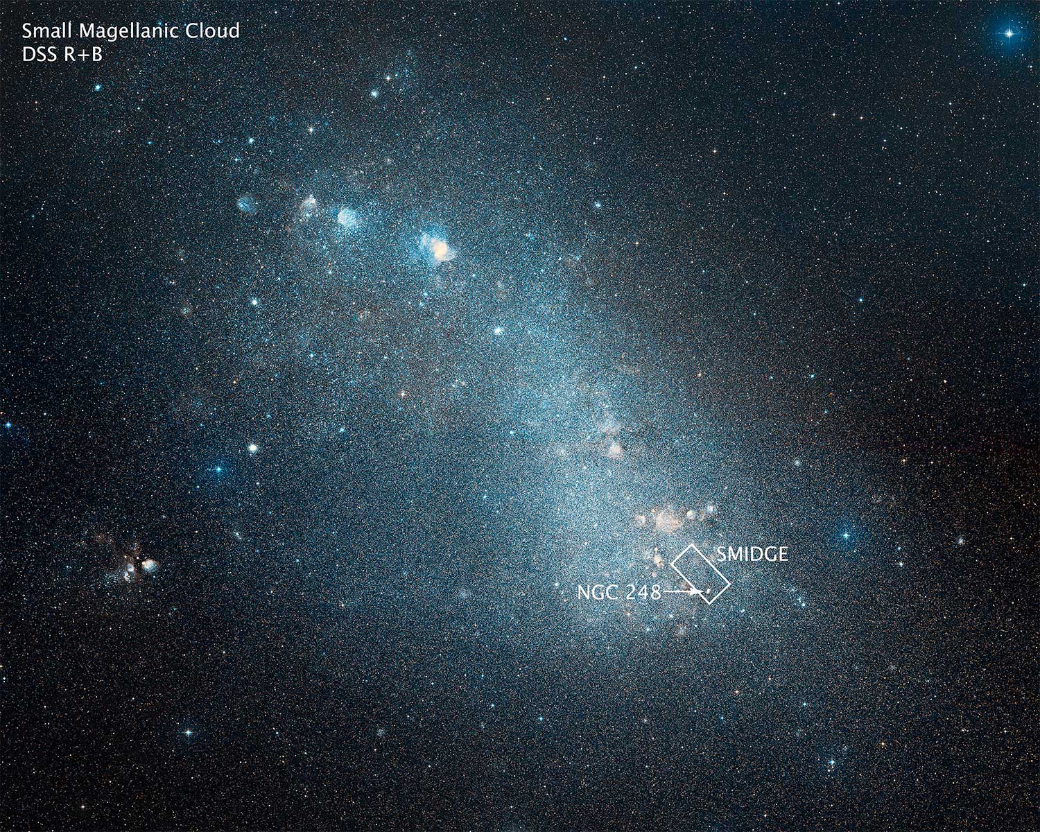
This ground-based image shows the Small Magellanic Cloud. The area of the SMIDGE survey is highlighted, as well as the position of NGC 248. Credit: NASA/ESA/Hubble/Digitized Sky Survey 2

However, there was something going on in the mass structure of M49 that astronomers were curious about… Something they couldn’t quite explain. Was it dark matter? As M. Lowenstein wrote in a 1992 study:

“An attempt to constrain the total mass distribution of the well-observed giant elliptical galaxy NGC 4472 is realized by constructing simultaneous equilibrium models for the gas and stars using all available relevant optical and X-ray data. The value of <?>, the emission-weighted average value of kT, derived from the Ginga spectrum, <?> = 1.9 ± 0.2 keV, can be reproduced only in hydrostatic models where nonluminous matter comprises at least 90% of the total mass. However, in general, these mass models are not consistent with observed projected stellar and globular cluster velocity dispersions at moderate radii.”

The next thing you know, nuclear outburst were discovered – the product of interaction with a neighboring galaxy. As B. Biller (et al) indicated in a 2004 study:

“We present the analysis of the Chandra ACIS observations of the giant elliptical galaxy NGC 4472. The Chandra Observatory’s arcsec resolution reveals a number of new features. Specifically: 1) an ~8 arc min streamer or arm (this corresponds to a linear size of 36 kpc) extending southwest of the galaxy and an assymetrical, somewhat truncated streamer to the northeast. Smaller, morphologically similar structures are observed in NGC 4636 and are explained as shocks from a nuclear outburst in the recent past. The larger size of the NGC 4472 streamers requires a correspondingly higher energy input compared to the NGC 4636 case. The asymmetry of the streamers may be due to the interaction of NGC 4472 with the ambient Virgo cluster gas. 2) A string of small, extended sources south of the nucleus. These sources may stem from an interaction of NGC 4472 with the galaxy UGC 7637. 3) X-ray cavities corresponding to radio lobes, where expanding radio plasma has evacuated the X-ray emitting gas. We also present a luminosity function for the X-ray point sources detected within NGC 4472 which we compare to that for other early type galaxies.”

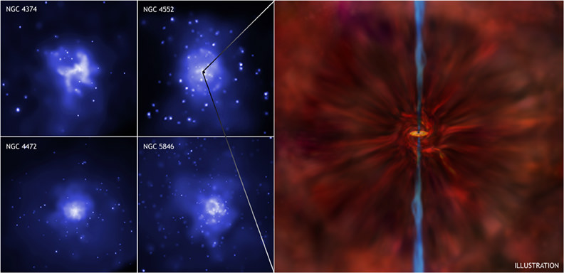
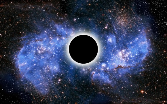
Chandra images showing 4 of the 9 galaxies discovered (left), and an artist’s impression on showing how gas falls towards a black hole and becomes a rapidly spinning disk of matter near the center (right). Credit: NASA/Chandra

But the very best was yet to come… the discovery of a black hole! According to NASA, the results from NASA’s Chandra X-ray Observatory, combined with new theoretical calculations, provide one of the best pieces of evidence yet that many supermassive black holes are spinning extremely rapidly. The images on the left show 4 out of the 9 large galaxies included in the Chandra study, each containing a supermassive black hole in its center.

The Chandra images show pairs of huge bubbles, or cavities, in the hot gaseous atmospheres of the galaxies, created in each case by jets produced by a central supermassive black hole. Studying these cavities allows the power output of the jets to be calculated. This sets constraints on the spin of the black holes when combined with theoretical models. The Chandra images were also used to estimate how much fuel is available for each supermassive black hole, using a simple model for the way matter falls towards such an object.

The artist’s impression on the right side of the main graphic shows gas within a “sphere of influence” falling straight inwards towards a black hole before joining a rapidly spinning disk of matter near the center. Most of the material in this disk is swallowed by the black hole, but some of it is swept outwards in jets (colored blue) by quickly spinning magnetic fields close to the black hole.

Previous work with these Chandra data showed that the higher the rate at which matter falls towards these supermassive black holes, the higher their power output is in jets. However, without detailed theory the implications of this result for black hole behavior were unclear. The new study uses these Chandra results combined with leading theoretical models for the production of jets, plus general relativity, to show that the supermassive black holes in these galaxies must be spinning at close to the maximum rate. If black holes are spinning at this limit, material can be dragged around them at close to the speed of light, the speed limit from Einstein’s theory of relativity.

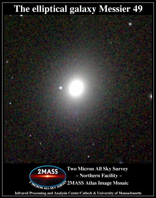
Atlas Image obtained of Messier 49, taken by the Two Micron All Sky Survey (2MASS). Credit: NASA/UofMass/IPAC/Caltech/NASA/NSF/2MASS

History of Observation:

According to SEDS, M49 was the first member of the Virgo cluster of galaxies to be discovered, by Charles Messier, who cataloged it on February 19th, 1771. As he recorded in his notes at the time:

“Nebula discovered near the star Rho Virginis. One cannot see it without difficulty with an ordinary telescope of 3.5-feet [FL]. The Comet of 1779 was compared by M. Messier with this nebula on April 22 and 23: The comet and the nebula had the same light. M. Messier has reported this nebula on the chart of the route of the comet, which appeared in the volume of the Academy of the same year 1779. Seen again on April 10, 1781.” Eight years later, on April 22, 1779, on the occasion of following the comet of that year, and on the hunt for finding more nebulous objects in competition to other observers, Barnabas Oriani independently rediscovered this ‘nebula’: “Very pale and looking exactly like the comet [1779 Bode, C/1779 A1].”

In his Bedford Catalogue of 1844, Admiral William H. Smyth confused this finding with Messier’s discovery:

“A bright, round, and well-defined nebula, on the Virgin’s left shoulder; exactly on the line between Delta Virginis and Beta Leonis, 8deg, or less than half-way, from the former star. With an eyepiece magnifying 93 times, there are only two telescopic stars in the field, one of which is in the sp and the other in the sf quadrant; and the nebula has a very pearly aspect. This object was discovered by Oriani in 1771 [this is wrong: it was Messier who discovered it that year; Oriani found it only in 1779], and registered by Messier as a “faint nebula, not seen without difficulty,” with a telescope of 3 1/2 feet in length. It is a pity that this active and very assiduous astronomer could not have been furnished with one of the giant telescopes of the present days. Had he possessed efficient means, there can be no doubt of the augmentation of his useful and, in its day, unique Catalogue: a collection of objects for which sidereal astronomy must ever remain indebted to him.” This error was repeated by John Herschel in his General Catalogue of 1864 (GC), who also erroneously assigned this object to “1771 Oriani,” and also found its way into J.L.E. Dreyer’s NGC.

Let’s hope you don’t mistake it with the many other galaxies nearby!

The location of Messier 49 within the Virgo constellation. Credit: IAU and Sky & Telescope magazine (Roger Sinnott & Rick Fienberg)

Locating Messier 49:

Galaxy hopping isn’t an easy chore and it takes some practice. Starting looking for M49 about halfway between Epsilon and Beta Virginis. Use Gamma to help triangulate your position. At near magnitude 8, Messier 49 is quite binocular possible and would show under dark sky conditions as a faint, very small egg shaped fog. However, it will not show in a finderscope of a telescope – but the nearby stars will.

Use their patterns to help guide you there. Because galaxies require dark skies, M49 cannot be found under urban conditions or during moonlit nights. In telescopes as small as 70mm, it will appear as a nebulous egg shape and become brighter – but no more resolved to larger instruments. To assist in location, begin with lowest magnification and increase magnification once found to darken background field.

And here are the quick facts to help you get started!

Object Name: Messier 49
Alternative Designations: M49, NGC 4472
Object Type: Elliptical Galaxy
Constellation: Virgo
Right Ascension: 12 : 29.8 (h:m)
Declination: +08 : 00 (deg:m)
Distance: 60000 (kly)
Visual Brightness: 8.4 (mag)
Apparent Dimension: 9×7.5 (arc min)

We have written many interesting articles about Messier Objects here at Universe Today. Here’s Tammy Plotner’s Introduction to the Messier Objects, , M1 – The Crab Nebula, M8 – The Lagoon Nebula, and David Dickison’s articles on the 2013 and 2014 Messier Marathons.

Be to sure to check out our complete Messier Catalog. And for more information, check out the SEDS Messier Database.

Sources:

• Messier Objects – Messier 49
• SEDS – Messier 49
• Wikipedia – Messier 49

The post Messier 49 – the NGC 4472 Elliptical Galaxy appeared first on Universe Today.

How Far Does Light Travel in a Year?

How Far Does Light Travel in a Year?:

The Universe is an extremely big place. As astronomers looked farther into space over the centuries, and deeper into the past, they came to understand just how small and insignificant our planet and our species seem by comparison. At the same time, ongoing investigations into electromagnetism and distant stars led scientists to deduce what the the speed of light is – and that it is the fastest speed obtainable.

As such, astronomers have taken to using the the distance light travels within a single year (aka. a light year) to measure distances on the interstellar and intergalactic scale. But how far does light travel in a year? Basically, it moves at a speed of 299,792,458 meters per second (1080 million km/hour; 671 million mph), which works out to about 9,460.5 billion km (5,878.5 billion miles) per year.

The Speed of Light:

Calculating the speed of light has been a preoccupation for scientists for many centuries. And prior to the 17th century, there was disagreement over whether the speed of light was finite, or if it moved from one spot to the next instantaneously. In 1676, Danish astronomer Ole Romer settled the argument when his observations of the apparent motion of Jupiter’s moon Io revealed that the speed of light was finite.

Light moves at different wavelengths, represented here by the different colors seen in a prism. Credit: NASA/ESA

From his observations, fellow Danish astronomer Christiaan Huygens calculated the speed of light at 220,000 km/s (136,701 mi/s). Over the course of the nest two centuries, the speed of light was refined further and further, producing estimates that ranged from about 299,000 to 315,000 km/s (185,790 to 195,732 mi/s).

This was followed by James Clerk Maxwell, who proposed in 1865 that light was an electromagnetic wave. In his theory of electromagnetism, the speed of light was represented as c. And then in 1905, Albert Einstein proposed his theory of Special Relativity, which postulated that the speed of light (c) was constant, regardless of the inertial reference frame of the observer or the motion of the light source.

By 1975, after centuries of refined measurements, the speed of light in a vacuum was calculated at 299,792,458 meters per second. Ongoing research also revealed that light travels at different wavelengths and is made up of subatomic particles known as photons, which have no mass and behave as both particles and waves.

Light-Year:

As already noted, the speed of light (expressed in meters per second) means that light travels a distance of 9,460,528,000,000 km (or 5,878,499,817,000 miles) in a single year. This distance is known as a “light year”, and is used to measure objects in the Universe that are at a considerable distances from us.

Examples of objects in our Universe, and the scale of their distances, based on the light year as a standard measure. Credit: Bob King.

For example, the nearest star to Earth (Proxima Centauri) is roughly 4.22 light-years distant. The center of the Milky Way Galaxy is 26,000 light-years away, while the nearest large galaxy (Andromeda) is 2.5 million light-years away. To date, the candidate for the farthest galaxy from Earth is MACS0647-JD, which is located approximately 13.3 billion light years away.

And the Cosmic Microwave Background, the relic radiation which is believed to be leftover from the Big Bang, is located some 13.8 billion light years away. The discovery of this radiation not only bolstered the Big Bang Theory, but also gave astronomers an accurate assessment of the age of the Universe. This brings up another important point about measuring cosmic distances in light years, which is the fact that space and time are intertwined.

You see, when we see the light coming from a distant object, we’re actually looking back in time. When we see the light from a star located 400 light-years away, we’re actually seeing light that was emitted from the star 400 years ago. Hence, we’re seeing the star as it looked 400 years ago, not as it appears today. As a result, looking at objects billions of light-years from Earth is to see billions of light-years back in time.

Yes, light travels at an extremely fast speed. But given the sheer size and scale of the Universe, it can still take billions of years from certain points in the Universe to reach us here on Earth. Hence why knowing how long it takes for light to travel a single year is so useful to scientists. Not only does it allow us to comprehend the scale of the Universe, it also allows us to chart the process of cosmic evolution.

We have written many articles about the speed of light here at Universe Today. Here’s How Far is a Light Year?, What is the Speed of Light?, How Much Stuff is in a Light Year?, How Does Light Travel?, and How Far Can You See in the Universe?

Want more info on light-years? Here’s an article about light-years for HowStuffWorks, and here’s an answer from PhysLink.

We’ve also recorded an episode of Astronomy Cast on this topic. Listen here, Episode 10: Measuring Distance in the Universe.

Sources:

• NASA – How Fast is the Speed of Light?
• NASA: Starchild – What is a Light-Year and How is it Measured?
• Wikipedia – Speed of Light
• UCR – How is the Speed of Light Measured?

The post How Far Does Light Travel in a Year? appeared first on Universe Today.

How Does Mercury Compare to Earth?

How Does Mercury Compare to Earth?:

Mercury was appropriately named after the Roman messenger of the Gods. This is owed to the fact that its apparent motion in the night sky was faster than that of any of the other planets. As astronomers learned more about this “messenger planet”, they came to understand that its motion was due to its close orbit to the Sun, which causes it to complete a single orbit every 88 days.

Mercury’s proximity to the Sun is merely one of its defining characteristics. Compared to the other planets of the Solar System, it experiences severe temperature variations, going from very hot to very cold. It’s also very rocky, and has no atmosphere to speak of. But to truly get a sense of how Mercury stacks up compared to the other planets of the Solar System, we need to a look at how Mercury compares to Earth.

Size, Mass and Orbit:

The diameter of Mercury is 4,879 km, which is approximately 38% the diameter of Earth. In other words, if you put three Mercurys side by side, they would be a little larger than the Earth from end to end. While this makes Mercury smaller than the largest natural satellites in our system – such as Ganymede and Titan – it is more massive and far more dense than they are.

Mercury, as imaged by the MESSENGER spacecraft, revealing parts of the never seen by human eyes. Image Credit: NASA/JHUAPL/Carnegie Institution of Washington

In fact, Mercury’s mass is approximately 3.3 x 10²³ kg (5.5% the mass of Earth) which means that its density – at 5.427 g/cm³ – is the second highest of any planet in the Solar System, only slightly less than Earth’s (5.515 g/cm³). This also means that Mercury’s surface gravity is 3.7 m/s², which is the equivalent of 38% of Earth’s gravity (0.38 g). This means that if you weighed 100 kg (220 lbs) on Earth, you would weigh 38 kg (84 lbs) on Mercury.

Meanwhile, the surface area of Mercury is 75 million square kilometers, which is approximately 10% the surface area of Earth. If you could unwrap Mercury, it would be almost twice the area of Asia (44 million square km). And the volume of Mercury is 6.1 x 10¹⁰ km³, which works out to 5.4% the volume of Earth. In other words, you could fit Mercury inside Earth 18 times over and still have a bit of room to spare.

In terms of orbit, Mercury and Earth probably could not be more different. For one, Mercury has the most eccentric orbit of any planet in the Solar System (0.205), compared to Earth’s 0.0167. Because of this, its distance from the Sun varies between 46 million km (29 million mi) at its closest (perihelion) to 70 million km (43 million mi) at its farthest (aphelion).

This puts Mercury much closer to the Sun than Earth, which orbits at an average distance of 149,598,023 km (92,955,902 mi), or 1 AU. This distance ranges from 147,095,000 km (91,401,000 mi) to 152,100,000 km (94,500,000 mi) – 0.98 to 1.017 AU. And with an average orbital velocity of 47.362 km/s (29.429 mi/s), it takes Mercury a total 87.969 Earth days to complete a single orbit – compared to Earth’s 365.25 days.

The Orbit of Mercury during the year 2006. Credit: Wikipedia Commons/Eurocommuter

However, since Mercury also takes 58.646 days to complete a single rotation, it takes 176 Earth days for the Sun to return to the same place in the sky (aka. a solar day). So on Mercury, a single day is twice as long as a single year. Meanwhile on Earth, a single solar day is 24 hours long, owing to its rapid rotation of 1674.4 km/h. Mercury also has the lowest axial tilt of any planet in the Solar System – approximately 0.027°, compared to Earth’s 23.439°.

Structure and Composition:

Much like Earth, Mercury is a terrestrial planet, which means it is composed of silicate minerals and metals that are differentiated between a solid metal core and a silicate crust and mantle. For Mercury, the breakdown of these elements is higher than Earth. Whereas Earth is primarily composed of silicate minerals, Mercury is composed of 70% metallic and 30% of silicate materials.

Also like Earth, Mercury’s interior is believed to be composed of a molten iron that is surrounded by a mantle of silicate material. Mercury’s core, mantle and crust measure 1,800 km, 600 km, and 100-300 km thick, respectively; while Earth’s core, mantle and crust measure 3478 km, 2800 km, and up to 100 km thick, respectively.

What’s more, geologists estimate that Mercury’s core occupies about 42% of its volume (compared to Earth’s 17%) and the core has a higher iron content than that of any other major planet in the Solar System. Several theories have been proposed to explain this, the most widely accepted being that Mercury was once a larger planet that was struck by a planetesimal that stripped away much of the original crust and mantle.

Internal structure of Mercury: 1. Crust: 100–300 km thick 2. Mantle: 600 km thick 3. Core: 1,800 km radius. Credit: MASA/JPL

Surface Features:

In terms of its surface, Mercury is much more like the Moon than Earth. It has a dry landscape pockmarked by asteroid impact craters and ancient lava flows. Combined with extensive plains, these indicate that the planet has been geologically inactive for billions of years.

Names for these features come from a variety of sources. Craters are named for artists, musicians, painters, and authors; ridges are named for scientists; depressions are named after works of architecture; mountains are named for the word “hot” in different languages; planes are named for Mercury in various languages; escarpments are named for ships of scientific expeditions, and valleys are named after radio telescope facilities.

During and following its formation 4.6 billion years ago, Mercury was heavily bombarded by comets and asteroids, and perhaps again during the Late Heavy Bombardment period. Due to its lack of an atmosphere and precipitation, these craters remain intact billions of years later. Craters on Mercury range in diameter from small bowl-shaped cavities to multi-ringed impact basins hundreds of kilometers across.

The largest known crater is Caloris Basin, which measures 1,550 km (963 mi) in diameter. The impact that created it was so powerful that it caused lava eruptions on the other side of the planet and left a concentric ring over 2 km (1.24 mi) tall surrounding the impact crater. Overall, about 15 impact basins have been identified on those parts of Mercury that have been surveyed.

Enhanced-color image of Munch, Sander and Poe craters amid volcanic plains (orange) near Caloris Basin. Credit: NASA/JHUAPL/Carnegie Institution of Washington

Earth’s surface, meanwhile, is significantly different. For starters, 70% of the surface is covered in oceans while the areas where the Earth’s crust rises above sea level forms the continents. Both above and below sea level, there are mountainous features, volcanoes, scarps (trenches), canyons, plateaus, and abyssal plains. The remaining portions of the surface are covered by mountains, deserts, plains, plateaus, and other landforms.

Mercury’s surface shows many signs of being geologically active in the past, mainly in the form of narrow ridges that extend up to hundreds of kilometers in length. It is believed that these were formed as Mercury’s core and mantle cooled and contracted at a time when the crust had already solidified. However, geological activity ceased billions of years ago and its crust has been solid ever since.

Meanwhile, Earth is still geologically active, owning to convection of the mantle. The lithosphere (the crust and upper layer of the mantle) is broken into pieces called tectonic plates. These plates move in relation to one another and interactions between them is what causes earthquakes, volcanic activity (such as the “Pacific Ring of Fire“), mountain-building, and oceanic trench formation.

Atmosphere and Temperature:

When it comes to their atmospheres, Earth and Mercury could not be more different. Earth has a dense atmosphere composed of five main layers – the Troposphere, the Stratosphere, the Mesosphere, the Thermosphere, and the Exosphere. Earth’s atmosphere is also primarily composed of nitrogen (78%) and oxygen (21%) with trace concentrations of water vapor, carbon dioxide, and other gaseous molecules.

The Fast Imaging Plasma Spectrometer on board MESSENGER has found that the solar wind is able to bear down on Mercury enough to blast particles from its surface into its wispy atmosphere. Credit: Shannon Kohlitz, Media Academica, LLC

Because of this, the average surface temperature on Earth is approximately 14°C, with plenty of variation due to geographical region, elevation, and time of year. The hottest temperature ever recorded on Earth was 70.7°C (159°F) in the Lut Desert of Iran, while the coldest temperature was -89.2°C (-129°F) at the Soviet Vostok Station on the Antarctic Plateau.

Mercury, meanwhile, has a tenuous and variable exosphere that is made up of hydrogen, helium, oxygen, sodium, calcium, potassium and water vapor, with a combined pressure level of about 10^-14 bar (one-quadrillionth of Earth’s atmospheric pressure). It is believed this exosphere was formed from particles captured from the Sun, volcanic outgassing and debris kicked into orbit by micrometeorite impacts.

Because it lacks a viable atmosphere, Mercury has no way to retain the heat from the Sun. As a result of this and its high eccentricity, the planet experiences far more extreme variations in temperature than Earth does. Whereas the side that faces the Sun can reach temperatures of up to 700 K (427° C), the side that is in darkness can reach temperatures as low as 100 K (-173° C).

Despite these highs in temperature, the existence of water ice and even organic molecules has been confirmed on Mercury’s surface. The floors of deep craters at the poles are never exposed to direct sunlight, and temperatures there remain below the planetary average. In this respect, Mercury and Earth have something else in common, which is the presence of water ice in its polar regions.

Mercury’s Magnetic Field. Credit: NASA

Magnetic Fields:

Much like Earth, Mercury has a significant, and apparently global, magnetic field, one which is about 1.1% the strength of Earth’s. It is likely that this magnetic field is generated by a dynamo effect, in a manner similar to the magnetic field of Earth. This dynamo effect would result from the circulation of the planet’s iron-rich liquid core.

Mercury’s magnetic field is strong enough to deflect the solar wind around the planet, thus creating a magnetosphere. The planet’s magnetosphere, though small enough to fit within Earth, is strong enough to trap solar wind plasma, which contributes to the space weathering of the planet’s surface.

All told, Mercury and Earth are in stark contrast. While both are terrestrial in nature, Mercury is significantly smaller and less massive than Earth, though it has a similar density. Mercury’s composition is also much more metallic than that of Earth, and its 3:2 orbital resonance results in a single day being twice as long as a year.

But perhaps most stark of all are the extremes in temperature variations that Mercury goes through compared to Earth. Naturally, this is due to the fact that Mercury orbits much closer to the Sun than the Earth does and has no atmosphere to speak of. And its long days and long nights also mean that one side is constantly being baked by the Sun, or in freezing darkness.

We have written many stories about Mercury on Universe Today. Here’s Interesting Facts About Mercury, What Type of Planet is Mercury?, How Long is a Day on Mercury?, The Orbit of Mercury. How Long is a Year on Mercury?, What is the Surface Temperature of Mercury?, Water Ice and Organics Found at Mercury’s North Pole, Characteristics of Mercury,, Surface of Mercury, and Missions to Mercury

If you’d like more information on Mercury, check out NASA’s Solar System Exploration Guide, and here’s a link to NASA’s MESSENGER Misson Page.

We have also recorded a whole episode of Astronomy Cast that’s just about planet Mercury. Listen to it here, Episode 49: Mercury.

Sources:

• NASA: Solar System Exploration – Mercury
• NASA – Mercury in Depth
• Wikipedia – Mercury
• Wikipedia – Earth

The post How Does Mercury Compare to Earth? appeared first on Universe Today.

Super-Earth Planet Found in the Habitable Zone of a Nearby Star

Super-Earth Planet Found in the Habitable Zone of a Nearby Star:

M-type stars, also known as “red dwarfs”, have become a popular target for exoplanet hunters of late. This is understandable given the sheer number of terrestrial (i.e. rocky) planets that have been discovered orbiting around red dwarf stars in recent years. These discoveries include the closest exoplanet to our Solar System (Proxima b) and the seven planets discovered around TRAPPIST-1, three of which orbit within the star’s habitable zone.

The latest find comes from a team of international astronomers who discovered a planet around GJ 625, a red dwarf star located just 21 light years away from Earth. This terrestrial planet is roughly 2.82 times the mass of Earth (aka. a “super-Earth”) and orbits within the star’s habitable zone. Once again, news of this discovery is prompting questions about whether or not this world could indeed be habitable (and also inhabited).

The international team was led by Alejandro Mascareño of the Canary Islands Institute of Astrophysics (IAC), and includes members from the University of La Laguna and the University of Geneva. Their research was also supported by the Spanish National Research Council (CSIS), the Institute of Space Studies of Catalonia (IEEC), and the National Institute For Astrophysics (INAF).

Diagram showing GJ 625’s habitable zone in comparison’s to the Sun’s. Credit: IAC

The study which details their findings was recently accepted for publication by the journal Astronomy & Astrophysics, and appears online under the title “A super-Earth on the Inner Edge of the Habitable Zone of the Nearby M-dwarf GJ 625“. According to the study, the team used radial-velocity measurements of GJ 625 in order to determine the presence of a planet that has between two and three times the mass of Earth.

This discovery was part of the HArps-n red Dwarf Exoplanet Survey (HADES), which studies red dwarf stars to determine the presence of potentially habitable planets orbiting them. This survey relies on the High Accuracy Radial velocity Planet Searcher for the Northern hemisphere (HARPS-N) instrument – which is part of the 3.6-meter Galileo National Telescope (TNG) at the IAC’s Roque de Los Muchachos Observatory on the island of La Palma.

Using this instrument, the team collected high-resolution spectroscopic data of the GJ 625 system over the course of three years. Specifically, they measured small variations in the stars radial velocity, which are attributed to the gravitational pull of a planet. From a total of 151 spectra obtained, they were able to determine that the planet (GJ 625 b) was likely terrestrial and had a minimum mass of 2.82 ± 0.51 Earth masses.

Moreover, they obtained distance estimates that placed it roughly 0.078 AU from its star, and an orbital period estimate of 14.628 ± 0.013 days. At this distance, the planet’s orbit places it just within GJ 625’s habitable zone. Of course, this does not mean conclusively that the planet has conditions conducive to life on its surface, but it is an encouraging indication.

Tjhe Observatorio del Roque de los Muchachos, located on the island of La Palma. Credit: IAC

As Alejandro Suárez Mascareño explained in an IAC press release:

“As GJ 625 is a relatively cool star the planet is situated at the edge of its habitability zone, in which liquid water can exist on its surface. In fact, depending on the cloud cover of its atmosphere and on its rotation, it could potentially be habitable”.

This is not the first time that the HADES project detected an exoplanet around a red dwarf star. In fact, back in 2016, a team of international researchers used this project to discover 2 super-Earths orbiting GJ 3998, a red dwarf located about 58 ± 2.28 light years from Earth. Beyond HADES, this discovery is yet another in a long line of rocky exoplanets that have been discovered in the habitable zone of a nearby red dwarf star.

Such findings are very encouraging since red dwarfs are the most common type of star in the known Universe- accounting for an estimated 70% of stars in our galaxy alone. Combined with the fact that they can exist for up to 10 trillion years, red dwarf systems are considered a prime candidate in the search for habitable exoplanets.

But as with all other planets discovered around red dwarf stars, there are unresolved questions about how the star’s variability and stability could affect the planet. For starters, red dwarf stars are known to vary in brightness and periodically release gigantic flares. In addition, any planet close enough to be within the star’s habitable zone would likely be tidally-locked with it, meaning that one side would be exposed to a considerable amount of radiation.

Artist’s impression of of the exoplanets orbiting a red dwarf star. Credit: ESO/M. Kornmesser/N. Risinger (skysurvey.org).

As such, additional observations will need to be made of this exoplanet candidate using the time-tested transit method. According to Jonay Hernández – a professor from the University of La Laguna, a researcher with the IAC and one of the co-authors on the study – future studies using this method will not only be able to confirm the planet’s existence and characterize it, but also determine if there are any other planets in the system.

“In the future, new observing campaigns of photometric observations will be essential to try to detect the transit of this planet across its star, given its proximity to the Sun,” he said. “There is a possibility that there are more rocky planets around GJ 625 in orbits which are nearer to, or further away from the star, and within the habitability zone, which we will keep on combing”.

According to Rafael Rebolo – one of the study’s co-authors from the Univeristy of La Laguna, a research with the IAC, and a member of the CSIS – future surveys using the transit method will also allow astronomers to determine with a fair degree of certainty whether or not GJ 625 b has the all-important ingredient for habitability – i.e. an atmosphere:

“The detection of a transit will allow us to determine its radius and its density, and will allow us to characterize its atmosphere by the transmitted light observe using high resolution high stability spectrographs on the GTC or on telescopes of the next generation in the northern hemisphere, such as the Thirty Meter Telescope (TMT)”.

Artist’s impression of a system of exoplanets orbiting a low mass, red dwarf star. Credit: NASA/JPL

But what is perhaps most exciting about this latest find is how it adds to the population of extra-solar planets within our cosmic neighborhood. Given their proximity, each of these planets represent a major opportunity for research. And as Dr. Mascareño told Universe Today via email:

“While we have already found more than 3600 extra-solar planets, the exoplanet population in our near neighborhood is still somewhat unknown. At 21 ly from the Sun, GJ 625 is one of the 100 nearest  stars, and right now GJ 625 b is one of the 30 nearest exoplanets detected and the 6th nearest potentially habitable exoplanet.”

Once again, ongoing surveys of nearby star systems is providing plenty of potential targets in the search for life beyond our Solar System. And with both ground-based and space-based next-generation telescopes joining the search, we can expect to find many, many more candidates in the coming years. In the meantime, be sure to check out this animation of GJ 625 b and its parent star:

Further Reading: arXiv, IAC

The post Super-Earth Planet Found in the Habitable Zone of a Nearby Star appeared first on Universe Today.

Best Jupiter Images From Juno … So Far

Best Jupiter Images From Juno … So Far:

The original plans for the Juno mission to Jupiter didn’t include a color camera. You don’t need color images when the mission’s main goals are to map Jupiter’s magnetic and gravity fields, determine the planet’s internal composition, and explore the magnetosphere.

But a camera was added to the manifest, and the incredible images from the JunoCam have been grabbing the spotlight.

As an instrument where students and the public can choose the targets, JunoCam is a “public outreach” camera, meant to educate and captivate everyday people.

“The whole endeavor of JunoCam was to get the public to participate in a meaningful way,” said Candy Hansen, Juno co-investigator at the Planetary Science Institute in Tucson, Arizona, speaking at a press conference last week to showcase Juno’s science and images.

And participate they have. Hundreds of ‘amateur’ image processing enthusiasts have been processing raw data from the JunoCam, turning them into stunning images, many reminiscent of a swirling Van Gogh ‘starry night’ or a cloudscape by Monet.

The swirling cloudtops of Jupiter, as seen by Juno during Perijove 5 on March 27, 2017. Credit: NASA/JPL-Caltech/SwRI/MSSS/Sophia Nasr.

“The contributions of the amateurs are essential,” Hansen said. “I cannot overstate how important the contributions are. We don’t have a way to plan our data without the contributions of the amateur astronomers. We don’t have a big image processing team, so we are completely relying on the help of our citizen scientists.”

Jupiter as seen by Juno during Perijove 6 in May, 2017. Credit: NASA/SwRI/MSSS/Gerald Eichstädt / Seán Doran.

Click on this image to have access to a 125 Megapixel upscaled print portrait.

Featured here are images processed by Seán Doran, Sophia Nasr, Kevin Gill and Jason Major. Like hundreds of others around the world, they anxiously await for data to arrive to Earth, where it is uploaded to the public Juno website. Then they set to work to turn the data into images.

“What I find the most phenomenal of all is that this takes real work,” Hansen said. “When you download a JunoCam image and process it, it’s not something you do in five minutes. The pictures that we get that people upload back onto our site, they’ve invested hours and hours of their own time, and then generously returned that to us.”

This video shows Juno’s trajectory from Perijove 6, and is based on work by Gerald Eichstädt, compiled and edited by Seán Doran. “This is real imagery projected along orbit trajectory,” Doran explained on Twitter.



Many of the images are shared on social media, but you can see the entire gallery of processed JunoCam images here. The Planetary Society also has a wonderful gallery of images processed by people around the world.

Intricate swirls on Jupiter Jupiter, from Juno’s Perijove 6 pass on May 19, 2017. Credit:
NASA/JPL-Caltech/SwRI /MSSS/Kevin M. Gill.

Details of Jupiter’s swirling gas clouds, as seen by Juno during the Perijove 6 pass in May, 2017. Credit:
NASA / SwRI / MSSS / Gerald Eichstädt / Seán Doran.

JunoCam was built by Malin Space Science Systems, which has cameras on previous missions like the Curiosity Mars Rover, the Mars Global Surveyor and the Mars Color Imager on the Mars Reconnaissance Orbiter. To withstand the harsh radiation environment at Jupiter, the camera required special protection and a reinforced lens.

Whenever new images arrive, many of us feel exactly like editing enthusiast Björn Jónsson:

I never expected I'd ever say this but: The latest @NASAJuno images of Jupiter are the most spectacular images of Jupiter I've ever seen. pic.twitter.com/7HawZ9RSwe

— Björn Jónsson (@bjorn_jons) May 25, 2017

Even the science team has expressed their amazement at these images.

“Jupiter looks different than what we expected,” said Scott Bolton, Juno’s principal investigator at the Southwest Research Institute. “Jupiter from the poles doesn’t look anything like it does from the equator. And the fact the north and south pole don’t look like each other, makes us wonder if the storms are stable, if they going to stay that way for years and years like the the Great Red Spot. Only time will tell us what is true.”

Read our article about the science findings from Juno.

A sequence of images of Jupiter from Juno’s Perijove 6 pass during May, 2017. Credit:
NASA / SwRI / MSSS / Gerald Eichstädt / Seán Doran.

Part of what makes these images so stunning is that Juno is closer to Jupiter than any previous spacecraft.

“Juno has an elliptical orbit that brings it between the inner edges of Jupiter’s radiation belt and the planet, passing only 5,000 km above the cloud tops,” Juno Project Manager Rick Nybakken told me in my book ‘Incredible Stories From Space: A Behind-the-Scenes Look at the Missions Changing Our View of the Cosmos.’ “This close proximity to Jupiter is unprecedented, as no other mission has conducted their science mission this close to the planet. We’re right on top of Jupiter, so to speak.”

Juno engineers designed the mission to enable the use of solar panels, which prior to Juno, have never been used on a spacecraft going so far from the Sun. Juno orbits Jupiter in a way that the solar panels are always pointed towards the Sun and the spacecraft never goes behind the planet. Juno’s orbital design not only enabled an historic solar-powered mission, it also established Juno’s unique science orbit.

White oval on Jupiter during Juno’s Perijove 4 pass on February 2, 2017. Processed from raw data. Credit: NASA/JPL-Caltech/SwRI/MSSS/Kevin M. Gill.

Uncalibrated, processed raw image from Juno’s Perijove 6 pass of Jupiter on May 19, 2017. Credit: NASA/SwRI/MSSS/Jason Major.

Juno spacecraft launched from Cape Canaveral on August 5, 2011. After traveling five years and 1.7 billion miles Juno arrived in orbit at Jupiter on July 4, 2016. The mission will last until at least February 2018, making 11 science orbits around Jupiter, instead of the 32 laps originally planned. Last year, engineers detected a problem with check valves in the propulsion system, and NASA decided to forego an engine burn to move Juno into a tighter 14-day orbit around Jupiter. The current 53.4 day orbit will be maintained, but depending on how the spacecraft responds, NASA could extend the mission another three years to give Juno more flybys near Jupiter.

The next science flyby will occur on July 11, when Juno will get some close-up views of the famous Great Red Spot.

Thanks to everyone who works on these images.

Animation of six images acquired by NASA’s Juno spacecraft on March 27, 2017. Credit: NASA/JPL-Caltech/SwRI/MSSS/Jason Major.

This enhanced color view of Jupiter’s south pole was created by citizen scientist Gabriel Fiset using data from the JunoCam instrument on NASA’s Juno spacecraft. Oval storms dot the cloudscape. Approaching the pole, the organized turbulence of Jupiter’s belts and zones transitions into clusters of unorganized filamentary structures, streams of air that resemble giant tangled strings. The image was taken on Dec. 11, 2016 at 9:44 a.m. PST (12:44 p.m. EST), from an altitude of about 32,400 miles (52,200 kilometers) above the planet’s beautiful cloud tops. Credits: NASA/JPL-Caltech/SwRI/MSSS/Gabriel Fiset

The post Best Jupiter Images From Juno … So Far appeared first on Universe Today.

What Exactly Should We See When a Star Splashes into a Black Hole Event Horizon?

What Exactly Should We See When a Star Splashes into a Black Hole Event Horizon?:

At the center of our Milky Way galaxy dwells a behemoth. An object so massive that nothing can escape its gravitational pull, not even light. In fact, we think most galaxies have one of them. They are, of course, supermassive black holes.

Supermassive black holes are stars that have collapsed into a singularity. Einstein’s General Theory of Relativity predicted their existence. And these black holes are surrounded by what’s known as an event horizon, which is kind of like the point of no return for anything getting too close to the black hole. But nobody has actually proven the existence of the event horizon yet.

Some theorists think that something else might lie at the center of galaxies, a supermassive object event stranger than a supermassive black hole. Theorists think these objects have somehow avoided a black hole’s fate, and have not collapsed into a singularity. They would have no event horizon, and would have a solid surface instead.

“Our whole point here is to turn this idea of an event horizon into an experimental science, and find out if event horizons really do exist or not,” – Pawan Kumar Professor of Astrophysics, University of Texas at Austin.

A team of researchers at the University of Texas at Austin and Harvard University have tackled the problem. Wenbin Lu, Pawan Kumar, and Ramesh Narayan wanted to shed some light onto the event horizon problem. They wondered about the solid surface object, and what would happen when an object like a star collided with it. They published their results in the Monthly Notices of the Royal Astronomical Society.

Artist’s conception of the event horizon of a black hole. Credit: Victor de Schwanberg/Science Photo Library

“Our whole point here is to turn this idea of an event horizon into an experimental science, and find out if event horizons really do exist or not,” said Pawan Kumar, Professor of Astrophysics at The University of Texas at Austin, in a press release.

Since a black hole is a star collapsed into a singularity, it has no surface area, and instead has an event horizon. But if the other theory turns out to be true, and the object has a solid surface instead of an event horizon, then any object colliding with it would be destroyed. If a star was to collide with this hard surface and be destroyed, the team surmised, then the gas from the star would enshroud the object and shine brightly for months, or even years.

This is the first in a sequence of two artist’s impressions that shows a huge, massive sphere in the center of a galaxy, rather than a supermassive black hole. Here a star moves towards and then smashes into the hard surface of the sphere, flinging out debris. The impact heats up the site of the collision. Image:
Mark A. Garlick/CfA

In this second artist’s impression a huge sphere in the center of a galaxy is shown after a star has collided with it. Enormous amounts of heat and a dramatic increase in the brightness of the sphere are generated by this event. The lack of observation of such flares from the center of galaxies means that this hypothetical scenario is almost completely ruled out. Image: Mark A. Garlick/CfA

If that were the case, then the team knew what to look for. They also worked out how often this would happen.

“We estimated the rate of stars falling onto supermassive black holes,” Lu said in the same press release. “Nearly every galaxy has one. We only considered the most massive ones, which weigh about 100 million solar masses or more. There are about a million of them within a few billion light-years of Earth.”

Now they needed a way to search the sky for these objects, and they found it in the archives of the Pan-STARRS telescope. Pan-STARRS is a 1.8 meter telescope in Hawaii. That telescope recently completed a survey of half of the northern hemisphere of the sky. In that survey, Pan-STAARS spent 3.5 years looking for transient objects in the sky, objects that brighten and then fade. They searched the Pan-STARR archives for transient objects that had the signature they predicted from stars colliding with these supermassive, hard-surfaced objects.



The trio predicted that in the 3.5 year time-frame captured by the Pan-STAARS survey, 10 of these collisions would occur and should be represented in the data.

“It turns out it should have detected more than 10 of them, if the hard-surface theory is true.” – Wenbin Lu, Dept. of Astronomy, University of Texas at Austin.

“Given the rate of stars falling onto black holes and the number density of black holes in the nearby universe, we calculated how many such transients Pan-STARRS should have detected over a period of operation of 3.5 years. It turns out it should have detected more than 10 of them, if the hard-surface theory is true,” Lu said.

The team found none of the flare-ups they expected to see if the hard-surface theory is true.

“Our work implies that some, and perhaps all, black holes have event horizons…” – Ramesh Narayan, Harvard-Smithsonian Center for Astrophysics.

What might seem like a failure, isn’t one of course. Not for Einstein, anyway. This represents yet another successful test of Einstein’s Theory of General Relativity, showing that the event horizon predicted in his theory does seem to exist.

As for the team, they haven’t abandoned the idea yet. In fact, according to Pawan Kumar, Professor of Astrophysics, University of Texas at Austin, “Our motive is not so much to establish that there is a hard surface, but to push the boundary of knowledge and find concrete evidence that really, there is an event horizon around black holes.”

“General Relativity has passed another critical test.” – Ramesh Narayan, Harvard-Smithsonian Center for Astrophysics.

“Our work implies that some, and perhaps all, black holes have event horizons and that material really does disappear from the observable universe when pulled into these exotic objects, as we’ve expected for decades,” Narayan said. “General Relativity has passed another critical test.”

The team plans to continue to look for the flare-ups associated with the hard-surface theory. Their look into the Pan-STARRS data was just their first crack at it.

An artist’s illustration of the Large Synoptic Survey Telescope with a simulated night sky. The team hopes to use the LSST to further refine their search for hard-surface supermassive objects. Image: Todd Mason, Mason Productions Inc. / LSST Corporation

They’re hoping to improve their test with the upcoming Large Synoptic Survey Telescope (LSST) being built in Chile. The LSST is a wide field telescope that will capture images of the night sky every 20 seconds over a ten-year span. Every few nights, the LSST will give us an image of the entire available night sky. This will make the study of transient objects much easier and effective.

More reading: Rise of the Super Telescopes: The Large Synoptic Survey Telescope

Sources:

• Do Stars Fall Quietly into Black Holes, or Crash into Something Utterly Unknown?
• Stellar disruption events support the existence of the black hole event horizon

The post What Exactly Should We See When a Star Splashes into a Black Hole Event Horizon? appeared first on Universe Today.

Flying Into the Sun? NASA’s Parker Solar Probe Mission

Flying Into the Sun? NASA’s Parker Solar Probe Mission:



If you’ve read enough of our articles, you know I’ve got an uneasy alliance with the Sun. Sure, it provides the energy we need for all life on Earth. But, it’s a great big ongoing thermonuclear reaction, and it’s right there! As soon as we get fusion, Sun, in like, 30 years or so, I tell you, we’ll be the ones laughing.

But to be honest, we still have so many questions about the Sun. For starters, we don’t fully understand the solar wind blasting out of the Sun. This constant wind of charged particles is constantly blowing out into space, but sometimes it’s stronger, and sometimes it’s weaker.

What are the factors that contribute to the solar wind? And as you know, these charged particles are not healthy for the human body, or for our precious electronics. In fact, the Sun occasionally releases enormous blasts that can damage our satellites and electrical grids.

How can we predict the intensity so that we can be better prepared for dangerous solar storms? Especially the Carrington-class events that might take down huge portions of our modern society.

Perhaps the biggest mystery with the Sun is the temperature of its corona. The surface of the Sun is hot, like 5,500 degrees Celsius. But if you rise up into the atmosphere of the Sun, into its corona, the temperature jumps beyond a million degrees.

The list of mysteries is long. And to start understanding what’s going on, we’ll need to get much much closer to the Sun.

Good news, NASA has a new mission in the works to do just that.

The Parker Solar Probe logo. Credit: NASA/JHUAPL

The mission is called the Parker Solar Probe. Actually, last week, it was called the Solar Probe Plus, but then NASA renamed it, and that reminded me to do a video on it.

It’s pretty normal for NASA to rename their spacecraft, usually after a dead astronomer/space scientist, like Kepler, Chandra, etc. This time, though, they renamed it for a legendary solar astronomer Eugene Parker, who developed much of our modern thinking on the Sun’s solar wind. Parker just turned 90 and this is the first time NASA has named it after someone living.

Anyway, back to the spacecraft.

The mission is due to launch in early August 2018 on a Delta IV Heavy, so we’re still more than a year away at this point. When it does, it’ll carry the spacecraft on a very unusual trajectory through the inner Solar System.

The problem is that the Sun is actually a very difficult place to reach. In fact, it’s the hardest place to get to in the entire Solar System.

Remember that the Earth is traveling around the Sun at a velocity of 30 km/s. That’s almost three times the velocity it takes to get into orbit. That’s a lot of velocity.

In order to be able to get anywhere near the Sun, the probe needs to shed velocity. And in order to do this, it’s going to use gravitational slingshots with Venus. We’ve talked about gravitational slingshots in the past, and how you can use them to speed up a spacecraft, but you can actually do the reverse.

The Parker Solar Probe will fall down into Venus’ gravity well, and give orbital velocity to Venus. This will put it on a new trajectory which takes it closer to the Sun. It’ll do a total of 7 flybys in 7 years, each of which will tweak its trajectory and shed some of that orbital momentum.

Parker Solar Probe’s trajectory including Venus flybys. Credit: NASA/JHUAPL

You know, trying to explain orbital maneuvering is tough. I highly recommend that you try out Kerbal Space Program. I’ve learned more about orbital mechanics by playing that game for a few months than I have in almost 2 decades of space journalism. Go ahead, try to get to the Sun, I challenge you.

Anyway, with each Venus flyby, the Parker Solar Probe will get closer and closer to the Sun, well within the orbit of Mercury. Far closer than any spacecraft has ever gotten to the Sun. At its closest point, it’ll only be 5.9 million kilometers from the Sun. Just for comparison, the Earth orbits at an average distance of about 150 million kilometers. That’s close.

And over the course of its entire mission, the spacecraft is expected to make a total of 24 complete orbits of the Sun, analyzing that plasma ball from every angle.

The orbit is also highly elliptical, which means that it’s going really really fast at its closest point. Almost 725,000 km/h.

In order to withstand the intense temperatures of being this close to the Sun, NASA has engineered the Parker Solar Probe to shed heat. It’s equipped with an 11.5 cm-thick shield made of carbon-composite. For that short time it spends really close to the Sun, the spacecraft will keep the shield up, blocking that heat from reaching the rest of its instruments.

And it’s going to get hot. We’re talking about more than 1,300 degrees Celsius, which is about 475 times as much energy as a spacecraft receives here on Earth. In the outer Solar System, the problem is that there just isn’t enough energy to power solar panels. But where Parker is going, there’s just too much energy.

Now we’ve talked about the engineering difficulties of getting a spacecraft this close to the Sun, let’s talk about the science.

Coronal holes are regions in the sun’s atmosphere or corona where solar plasma can stream directly into space. Often a hole will a couple rotations, inciting repeat auroras approximately every 4 weeks. Credit: NASA

The biggest question astronomers are looking to solve is, how does the corona get so hot. The surface is 5,500 Celsius. As you get farther away from the Sun, you’d expect the temperature to go down. And it certainly does once you get as far as the orbit of the Earth.

But the Sun’s corona, or its outer atmosphere, extends millions of kilometers into space. You can see it during a solar eclipse as this faint glow around the Sun. Instead of dropping, the temperature rises to more than a million degrees.

What could be causing this? There are a couple of ideas. Plasma waves pushed off the Sun could bunch up and release their heat into the corona. You could also get the crisscrossing of magnetic field lines that create mini-flares within the corona, heating it up.

The second great mystery is the solar wind, the stream of charged protons and electrons coming from the Sun. Instead of a constant blowing wind, it can go faster or slower. And when the speed changes, the contents of the wind change too.

There’s the slow wind, that goes a mere 1.1 million km/h and seems to emanate from the Sun’s equatorial regions. And then the fast wind, which seems to be coming out of coronal holes, cooler parts in the Sun’s corona, and can be going at 2.7 million km/h.

Why does the solar wind speed change? Why does its consistency change?

Parker Solar Probe’s instruments. Credit: NASA/JHUAPL

The Parker Solar Probe is equipped with four major instruments, each of which will gather data from the Sun and its environment.

The FIELDS experiment will measure the electric and magnetic fields and waves around the Sun. We know that much of the Sun’s behavior is driven by the complex interaction between charged plasma in the Sun. In fact, many physicists agree that magnetohydrodynamics is easily one of the most complicated fields you can get into.

Integrated Science Investigation of the Sun, or ISOIS (which I suspect needs a renaming) will measure the charged particles streaming off the Sun, during regular solar activity and during dangerous solar storms. Can we get any warning before these events occur, giving astronauts more time to protect themselves?

Wide-field Imager for Solar PRobe or WISPR is its telescope and camera. It’s going to be taking close up, high resolution images of the Sun and its corona that will blow our collective minds… I hope. I mean, if it’s just a bunch of interesting data and no pretty pictures, it’s going to be hard to make cool videos showcasing the results of the mission. You hear me NASA, we want pictures and videos. And science, sure.

And then the Solar Wind Electrons Alphas and Protons Investigation, or SWEAP, will measure type, velocity, temperature and density of particles around the Sun, to help us understand the environment around it.

One interesting side note, the spacecraft will be carrying a tiny chip on board with photos of Eugene Parker and a copy of his original 1958 paper explaining the Sun’s solar wind.

The Parker Solar Probe orbiting the Sun. Credit: NASA/JHUAPL

I know we’re still more than a year away from liftoff, and several years away before the science data starts pouring in. But you’ll be hearing more and more about this mission shortly, and I’m pretty excited about what it’s going to accomplish. So stay tuned, and once the science comes in, I’m sure you’ll hear plenty more about it.

The post Flying Into the Sun? NASA’s Parker Solar Probe Mission appeared first on Universe Today.

The Sun Probably Lost a Binary Twin Billions of Years Ago

The Sun Probably Lost a Binary Twin Billions of Years Ago:

For us Earthlings, life under a single Sun is just the way it is. But with the development of modern astronomy, we’ve become aware of the fact that the Universe is filled with binary and even triple star systems. Hence, if life does exist on planets beyond our Solar System, much of it could be accustomed to growing up under two or even three suns. For centuries, astronomers have wondered why this difference exists and how star systems came to be.

Whereas some astronomers argue that individual stars formed and acquired companions over time, others have suggested that systems began with multiple stars and lost their companions over time. According to a new study by a team from UC Berkeley and the Harvard-Smithsonian Center for Astrophysics (CfA), it appears that the Solar System (and other Sun-like stars) may have started out as binary system billions of years ago.

This study, titled “Embedded Binaries and Their Dense Cores“, was recently accepted for publication in the Monthly Notices of the Royal Astronomical Society. In it, Sarah I. Sadavoy – a radio astronomer from the Max Planck Institute for Astronomy and the CfA – and Steven W. Stahler (a theoretical physicist from UC Berkeley) explain how a radio surveys of a star nursery led them to conclude that most Sun-like stars began as binaries.

The dark molecular cloud, Barnard 68, is a stellar nursery that can only be studied using radio astronomy. Credit: FORS Team, 8.2-meter VLT Antu, ESO

They began by examining the results of the first radio survey of the giant molecular cloud located about 600 light-years from Earth in the Perseus constellation – aka. the Perseus Molecular Cloud. This survey, known as the VLA/ALMA Nascent Disk and Multiplicity (VANDAM) survey, relied the Very Large Array in New Mexico and the Atacama Large Millimeter/submillimeter Array (ALMA) in Chile to conduct the first survey of the young stars (<4 million years old) in this star-forming region.

For several decades, astronomers have known that stars are born inside “stellar nurseries”, which are the dense cores that exist within immense clouds of dust and cold, molecular hydrogen. These clouds look like holes in the star field when viewed through an optical telescope, thanks to all the dust grains that obscure light coming from the stars forming within them and from background stars.

Radio surveys are the only way to probe these star-forming regions, since the dust grains emit radio transmissions and also do not block them. For years, Stahler has been attempting to get radio astronomers to examine molecular clouds in the hope of gathering information on the formation of young stars inside them. To this end, he approached Sarah Sadavoy – a member of the VANDAM team – and proposed a collaboration.

The two began their work together by conducting new observations of both single and binary stars within the dense core regions of the Perseus cloud. As Sadavoy explained in a Berkeley News press release, the duo were looking for clues as to whether young stars formed as individuals or in pairs:

“The idea that many stars form with a companion has been suggested before, but the question is: how many? Based on our simple model, we say that nearly all stars form with a companion. The Perseus cloud is generally considered a typical low-mass star-forming region, but our model needs to be checked in other clouds.”

Infrared image from the Hubble Space Telescope, showing a bright, fan-shaped object (lower right quadrant) thought to be a binary star that emits light pulses as the two stars interact. Credit: NASA/ESA/ J. Muzerolle (STScI)

Their observations of the Perseus cloud revealed a series of Class 0 and Class I stars – those that are <500,000 old and 500,000 to 1 million years old, respectively – that were surrounded by egg-shaped cocoons. These observations were then combined with the results from VANDAM and other surveys of star forming regions – including the Gould Belt Survey and data gathered by SCUBA-2 instrument on the James Clerk Maxwell Telescope in Hawaii.

From this, they created a census of stars within the Perseus cloud, which included 55 young stars in 24 multiple-star systems (all but five of them binary) and 45 single-star systems. What they observed was that all of the widely separated binary systems – separated by more than 500 AU – were very young systems containing two Class 0 stars  that tended to be aligned with the long axis of their egg-shaped dense cores.

Meanwhile, the slightly older Class I binary stars were closer together (separated by about 200 AU) and did not have the same tendency as far as their alignment was concerned. From this, the study’s authors began mathematically modelling multiple scenarios to explain this distribution, and concluded that all stars with masses comparable to our Sun start off as wide Class 0 binaries. They further concluded that 60% of these split up over time while the rest shrink to form tight binaries.

“As the egg contracts, the densest part of the egg will be toward the middle, and that forms two concentrations of density along the middle axis,” said Stahler. “These centers of higher density at some point collapse in on themselves because of their self-gravity to form Class 0 stars. “Within our picture, single low-mass, sunlike stars are not primordial. They are the result of the breakup of binaries. ”

The two brightest stars of the Centaurus constellation, the binary star system of Alpha Centauri. Credit: Wikipedia Commons/Skatebiker

Findings of this nature have never before been seen or tested. They also imply that each dense core within a stellar nursery (i.e. the egg-shaped cocoons, which typically comprise a few solar masses) converts twice as much material into stars as was previously thought. As Stahler remarked:

“The key here is that no one looked before in a systematic way at the relation of real young stars to the clouds that spawn them. Our work is a step forward in understanding both how binaries form and also the role that binaries play in early stellar evolution. We now believe that most stars, which are quite similar to our own sun, form as binaries. I think we have the strongest evidence to date for such an assertion.”

This new data could also be the start of a new trend, where astronomers rely on radio telescopes to examine dense star-forming regions with the hopes of witnessing more in the way of stellar formations. With the recent upgrades to the VLA and the Atacama Large Millimeter/submillimeter Array (ALMA) in Chile, and the ongoing data provided by the SCUBA-2 survey in Hawaii, these studies may be coming sooner other than later.

Another interesting implication of the study has to do with something known as the “Nemesis hypothesis”. In the past, astronomers have conjectured that a companion star named “Nemesis” existed within our Solar System. This star was so-named because the theory held that it was responsible for kicking the asteroid which caused the extinction of the dinosaurs into Earth’s orbit. Alas, all attempts to find Nemesis ended in failure.

Artist’s impression of the binary star system of Sirius, a white dwarf star in orbit around Sirius (a white supergiant). Credit: NASA, ESA and G. Bacon (STScI)

As Steven Stahler indicated, these findings could be interpreted as a new take on the Nemesis theory:

“We are saying, yes, there probably was a Nemesis, a long time ago. We ran a series of statistical models to see if we could account for the relative populations of young single stars and binaries of all separations in the Perseus molecular cloud, and the only model that could reproduce the data was one in which all stars form initially as wide binaries. These systems then either shrink or break apart within a million years.”

So while their results do not point towards a star being around for the extinction of the dinosaurs, it is possible (and even highly plausible) that billions of years ago, the Solar planets orbited around two stars. One can only imagine what implications this could have for the early history of the Solar System and how it might have affected planetary formation. But that will be the subject of future studies, no doubt!

Further Reading: Berkeley News, arXiv

The post The Sun Probably Lost a Binary Twin Billions of Years Ago appeared first on Universe Today.